Deep RL 10 Model-based Reinforcement Learning

Previous lecture is mainly about how to plan actions to take when the dynamics is known. In this lecture, we study how to learn the dynamics. We will also introduce how to incorporate planning in the model learning process and therefore form a complete decision making algorithm.

Again, most of the algorithms will be introduced in the context of deterministic dynamics, i.e. \(s_{t+1} = f(s_t, a_t)\), but almost all of these algorithms can just as well be applied in the stochastic dynamics setting, i.e. \(s_{t+1}\sim p(s_{t+1}\mid s_t, a_t)\), and when the distinction is salient, I’ll make it explicit.

1 Basic Model-based RL

How to learn a model, the most direct way is supervised learning. Similar to the idea used before, we run a random policy to get transitions, and then fit a neural net to the transition:

1. run base policy \(\pi_0(a\mid s)\) (e.g. random policy) to collect \(\mathcal{D} = \{ (s_i, a_i, s'_i) \}\)
2. learn dynamics model \(f_{\theta}(s,a)\) to minimize \(\sum_{i}\left\| s'_i - f_{\theta}(s_i, a_i) \right\|^2\)
3. plan through \(f_{\theta}(s,a)\) to choose actions.

Where in step 3, we can use CEM, MCTS, LQR etc.

Does this work? Well, in some cases. For example, if we have a full physics model of the dynamics and only need to fit a few parameters, this method can work. But still, some care should be taken to design a good base policy.

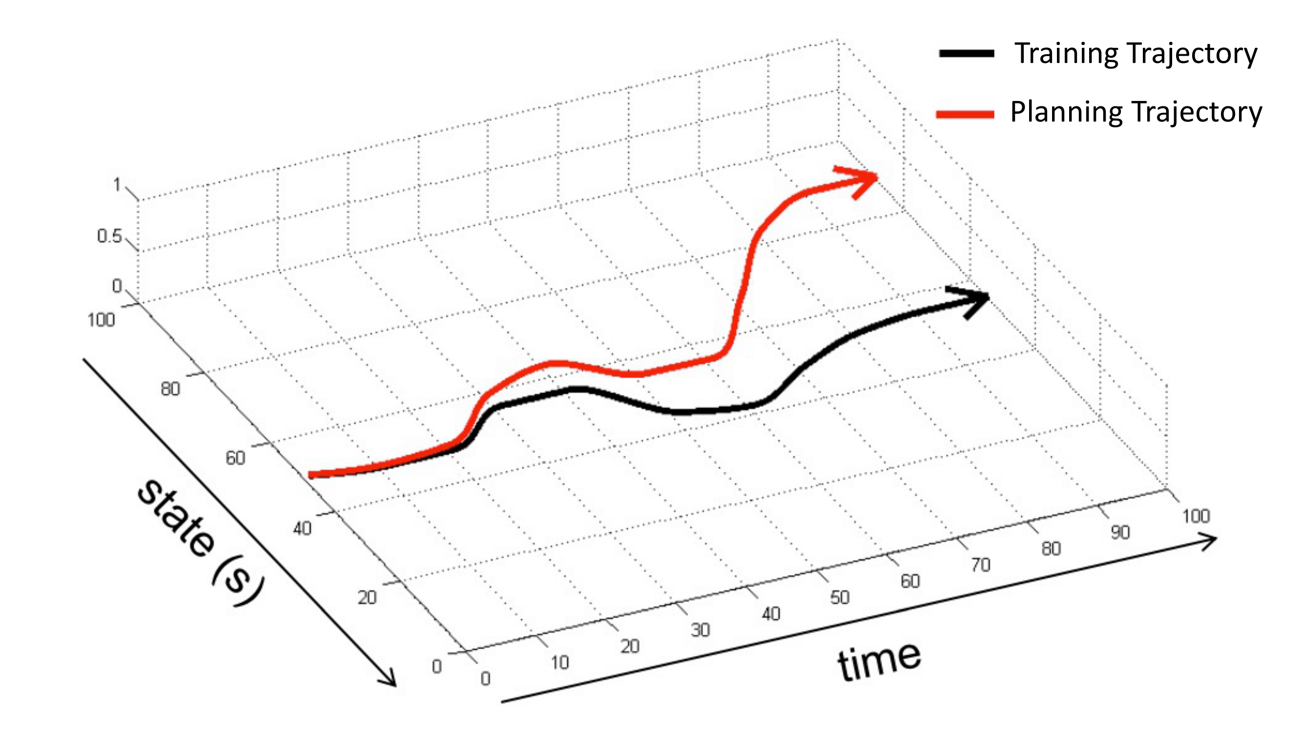
In general, however, this doesn’t workm and the reason is very similar to the one we encountered in imitation learning — distribution shift. The data we used to learn the dynamics comes from the trajectory distribution induced by random policy \(\pi_0\), but when we plan through the model, we can think of the algorithm is using another policy \(\pi_f\), and the trajectory distribution induced by this policy can be very different from the one induced by the base policy. The consequence is that, when we plan actions, we’ll arrive at the state action pair that the dynamics is very uncertain about, because it has never trained on similar data! Therefore, it will make bad prediction on the following state, which will in turn lead to bad actions, this will go on and on and in the end we are completely planning on the wrong states (prediction is different the reality). The intuitive plot is shown below:

How to deal with it? Same as how DAgger deals with distribution shift in imitation learning, we just need to make sure that the training data comes from the current dynamics (current policy). These lead to the first practical model-based RL algorithm:

1. run base policy \(\pi_0(a\mid s)\) (e.g. random policy) to collect \(\mathcal{D} = \{ (s_i, a_i, s'_i) \}\)
2. learn dynamics model \(f_{\theta}(s,a)\) to minimize \(\sum_{i}\left\| s'_i - f_{\theta}(s_i, a_i) \right\|^2\)
3. plan through \(f_{\theta}(s,a)\) to choose actions.
4. execute those actions and add the resulting transitions \(\{ (s_j, a_j, s'_j) \}\) to \(\mathcal{D}\). Go to step 2.

However, even though the data is updating based on the learned dynamics, as long as we are replanning, it will always induce a new trajectory distribution which will be a little different from the previous distribution. In another word, the distribution shift will always exist. Therefore, as we plan through \(f_{\theta}(s,a)\), the actual trajectory will gradually deviate from the predicted trajectory which will lead to bad actions.

We can improve this algorithm by only execute the first planned action, and observe the next state that this action leads to, and then replan start from that state. and then take the first action etc. In a word, at each step, we only take the first planned action and observe the state and then replan from there. Because at each time step, we always take the action based on the actual state, this is more reliable than executing the whole plan actions all in one go. The algorithm is

1. run base policy \(\pi_0(a\mid s)\) (e.g. random policy) to collect \(\mathcal{D} = \{ (s_i, a_i, s'_i) \}\)
2. learn dynamics model \(f_{\theta}(s,a)\) to minimize \(\sum_{i}\left\| s'_i - f_{\theta}(s_i, a_i) \right\|^2\)
3. plan through \(f_{\theta}(s,a)\) to choose actions.
4. execute the first planned action and add the resulting transition \((s, a, s)\) to \(\mathcal{D}\). If reach the predefined maximal number of planning steps, go to step 2; else, Go to step 3.

This algorithm is call Model Predictive Control or MPC. Replanning at each time step can drastically increase the computation load, so people sometimes choose to shorten the time horizon of the trajectory. While this might lead to a decrease in the quality of actions, since we are constantly replanning, we can take the cost that individual plans is less perfect.

2 Uncertainty-Aware Model-based RL

Since we plan actions replying on the fitted dynamics, whether or not the dynamics is a good representation of the world is crucial. When we use high capacity model like neural networks, we usually need to feed it with a lot of data in order to get a good fit. But in model-based RL, we usually don’t have a lot of data at the beginning, in fact, we can only have some bad data (generated by running some random policy), and then if we use neural network to fit the dynamics, it will overfit the data, and not have a good representation of the good part of the world. This will lead the algorithm to take bad actions, which can lead to bad states, which can then lead to neural net dynamics trained only on trajectories and thus it’s predictions on good states in unreliable, which again lead to algorithm to take bad actions…… This seems to be a chicken-and-egg problem, but if you think about it, the origin is that planning on unconfident state prediction can lead to bad actions.

The solution is to quantify uncertainty of the model, and take into consideration this uncertain in planning.

First of all, it’s important to know that uncertainty of a model is not the same thing as the probability of the model’s prediction on some state. Uncertainty is not about the setting where dynamics is noisy, but about the setting where we don’t know what the dynamics are.

The way to avoid taking risky actions on uncertain state is to plan based on expected expected reward. Wait, what is it? Yes, this is not a typo, the first expected is with respect to the model uncertainty, and the second expected is with respect to trajectory distribution. Mathematically, the objective is

\[\begin{align} &\int \int \sum_t r(s_t, a_t) p_{\theta}(\tau) p(\theta) \text{d}\tau \text{d}\theta \\ &= \int \left[\mathbb{E}_{\tau\sim p_{\theta}(\tau)}\sum_t r(s_t, a_t)\right] p(\theta)\text{d}\theta \\ &= \mathbb{E}_{\theta\sim p(\theta)}\left[ \mathbb{E}_{\tau\sim p_{\theta}(\tau)}\sum_t r(s_t, a_t) \right] \end{align}\]

Having an uncertainty-aware formulation, the next steps are:

1. how to get \(p(\theta)\)
2. how to actually plan actions to optimize this objective

2.1 Uncertainty-Aware Neural Networks

In this subsection we discuss how to get \(p(\theta)\). First of all, we should make sure that the general direction is to learn \(p(\theta)\) from data, thus we should explicitly write it as \(p(\theta\mid \mathcal{D})\) where \(\mathcal{D}\) is the data.

The first approach is Bayesian Neural Networks, or BNN. To consider the problem from a Bayesian perspective, we can first rethink our original approach, i.e. what is it that we are estimating when doing supervised training in step 2 in MPC? (Here we write it slightly differently for illustration)

learn dynamics model \(f_{\theta^*}(s,a)\) to minimize \(\sum_{i}\left\| s'_i - f_{\theta}(s_i, a_i) \right\|^2\)

The \(\theta\) that we find are actually the maximal likelihood estimation, i.e.

\[\theta^* = \text{argmax}_{\theta}p(\mathcal(D)\mid \theta)\]

Adopting the Bayesian approach, we want to estimate the posterior distribution

\[\begin{align*} p(\theta\mid \mathcal{D}) =\frac{p(\mathcal(D)\mid \theta)p(\theta)}{p(\mathcal{D})} \end{align*}\]

However, this calculation is usually intractable. In neural network setting, people usually resort to variance inference, which approaximates the intractable true \(p(\theta\mid \mathcal{D})\) by a tractable variational posterior \(p(\theta\mid\phi)\) by minimizing the Kullback-Leibler divergence (KL divergence)between the ground truth and approximation, where \(\phi\) is to be learned from data. We will introduce variational inference in future lectures, for now, we give a simple hand wavie example.

We define variational posterior to be fully factorized Gaussian:

\[p(\theta \mid \phi) = \prod N(\theta_j \mid \mu_j, \sigma^2_j)\]

Where \(\mu_j\) and \(\sigma^2_j\) are learned s.t. the variational posterior is close to the true posterior. Then we use \(p(\theta \mid \phi)\) as the distribution over dynamics and take actions accrodingly.

The second approach, which is conceptually simpler and usually works better than BNN, is boostrap ensembles. The idea is to train many independent neural dynamics models, and average them. Mathematically, we learn independent neural network parameters \(\theta_1, \theta_2, \cdots, \theta_m\) and the ensembled dynamics is

\[p(\theta\mid \mathcal{D}) = \frac1m sum_{j=1}^{m}\delta(\theta_j)\]

Where \(\delta\) is the delta function, and the probability of state \(s_{t+1}\) from the dynamics ensemble is an average of the probabilities of each independent neural dynamics:

\[\begin{align} \int p(s_{t+1}\mid s_t, a_t, \theta)p(\theta\mid \mathcal{D}) \text{d}\theta = \frac1m \sum_{j=1}^m p(s_{t+1}\mid s_t, a_t, \theta_j) \end{align}\]

But how do we get the \(m\) independent neural dynamics? We use boostrap. The idea is to resample the dataset \(\mathcal{D}\) with replacement to get \(m\) dataset and for each of the \(m\) dataset, train a dynamics. The bootstrap method is developed by statistician Bradley Efron since 1979. It has solid statistical foundation and has been applied to many areas. I encourage interested reader checkout this book by Efron and Tibshirani.

In practice, people find that for neural dynamics, it is not necessary to resample the data. What people do is just train neural nets with same dataset but set different random seed. The use of SGD will make each neural net sufficiently independent.

2.2 Plan with Uncertainty

Having uncertainty-aware dynamics i.e. a distribution over dynamics. It’s very natural to derive an uncertainty-aware MPC algorithm. Recall that in the MPC algorithm, we plan using the objective

\[J(a_1, \cdots, a_T) = \sum_{t=1}^{T}r(s_t, a_t), s_t = f_{\theta}(s_{t-1}, a_{t-1})\]

Now the objective has changed to

\[\begin{align}\label{un_obj} &J(a_1, \cdots, a_T) = \frac1m \sum_{j=1}^{m}\sum_{t=1}^{T}r(s_{t,j}, a_t)\\ &\text{ where } s_{t,j} = f_{\theta_j}(s_{t-1,j}, a_{t-1}) \text{ or } s_{t,j} \sim p(s_t\mid s_{t-1,j}, a_{t-1}, \theta_j)\\ &\text{ and } \theta_j \sim p(\theta\mid \mathcal{D}) \end{align}\]

With this, we can write out the uncertainty-aware MPC algorithm:

1. run base policy \(\pi_0(a\mid s)\) (e.g. random policy) to collect \(\mathcal{D} = \{ (s_i, a_i, s'_i) \}\)
2. estimate the posterior distirbution of dynamics parameters \(p(\theta\mid \mathcal{D})\)
3. sample \(m\) dynamics from \(p(\theta\mid \mathcal{D})\)
4. plan through the ensemble dynamics to choose actions.
5. execute the first planned action and add the resulting transition \((s, a, s)\) to \(\mathcal{D}\). If reach the predefined maximal number of planning steps, go to step 2; else, Go to step 3.

You might notice that this algorithm seems do not use the objective i.e. equation \(\ref{un_obj}\), but actually at step 4, the algorithm is actually planning based on equation \(\ref{un_obj}\), and since the reward relies on ensemble dynamics, we conveniently say “plan through the ensemble dynamics to choose actions”.

3 Model-Based RL with Images

Previously we’ve been assuming that state is obserable, because we’ve been using transitions \(\{ (s_i, a_i, s'_i) \}\) for supervised learning of dynamics (or distribution of dynamics). In some cases, especially when the observation is image, directly treating it as state for supervised learning of dynamics can be troublesome, and the reasons are:

1. High dimensionality. We are fitting \(s_{t+1} = f_{\theta}(s_t, a_t) \text{ or } s_{t+1} \sim p_{\theta}(s_{t+1}\mid s_t, a_t)\), if \(s_{t+1}\) is image, then the dimension is \(3\times\text{H}\times\text{W}\), which can be very large in many cases and thus accurate prediction is very difficult.
2. Redundancy. Many parts of the images can stay unchanged during the whole process, this leads a redundancy in the data.
3. Partial observability. There are things that static images can not directly represent, such as speed and acceleration, although you might derive this from the image, but that requires extra potentially nontrivial effort and might not be accurate.

We will now introduce the state-space model that models POMDPs, which treats states as latent variables and model observation using distributions conditioned on states.

Let’s recall how dynamics is learned when we assume states are observable. We parameterize the dynamics using a neural net with parameter \(\theta\):

\[p(s_{1:T}) = \prod_{t=1}^{T}p_{\theta}(s_{t+1}\mid s_t, a_t)\]

Note that we slightly abuse the notation for clarity, for example \(p_{\theta}(s_{1}\mid s_0, a_0) = p_{\theta}(s_1)\).

And solve for \(\theta\) using maximal likelihood on collected transitions \(\{ (s^i_{t+1}, s^i_t, a^i_t) \}_{i,t=1}^{N,T}\):

\[\max_{\theta}\frac1N \sum_{i=1}^{N} \sum_{t=1}^{T} \log p_{\theta}(s^i_{t+1}\mid s^i_t, a^i_t)\]

Now consider state unobservable, We have:

\[p(s_{1:T}, o_{1:T}) = \prod_{t=1}^{T}p_{\theta}(s_{t+1}\mid s_t, a_t)p_{\phi}(o_t\mid s_t)\]

Where \(p_{\theta}(s_{t+1}\mid s_t, a_t)\) is the transition model and \(p_{\phi}(o_t\mid s_t)\) is the observation model. Similarly, we solve for \(\theta \text{and} \phi\) using maximal likelihood

\[\begin{align} &\log \prod_{t=1}^{T} p_{\phi}(o_{t}\mid s_t) \nonumber \\ &=\log \mathbb{E}_{(s_t, s_{t+1}) \sim p(s_t, s_{t+1}\mid o_{1:t}, a_{1:t})}\prod_{t=1}^{T} p_{\theta}(s_{t+1}\mid s_t, a_t) p_{\phi}(o_{t}\mid s_t) \nonumber \\ &\geq \mathbb{E}_{(s_t, s_{t+1}) \sim p(s_t, s_{t+1}\mid o_{t}, a_{t})} \log \prod_{t=1}^{T} p_{\theta}(s_{t+1}\mid s_t, a_t) p_{\phi}(o_{t}\mid s_t) \nonumber \\ &\approx \frac1N \sum_{i=1}^{N} \sum_{t=1}^{T} \log p_{\theta}(s^i_{t+1}\mid s^i_t, a^i_t)+ \log p_{\phi}(o^i_{t}\mid s^i_t) \label{latent_obj} \end{align}\]

We maximize equation \(\ref{latent_obj}\), which is lower bound of the log likelihood, it actually uses one sample estimation for estimating the expectation (in terms of \((s_t, s_{t+1})\)), more sample can be used.

One issue is that by Bayes’ rule,

\[\begin{align} &p(s_t, s_{t+1}\mid o_{t}, a_{t}) \\ &= p_{\theta}(s_{t+1}\mid s_t, a_t) p(s_t\mid o_t) \\ &= p_{\theta}(s_{t+1}\mid s_t, a_t) \frac{ p_{\phi}(o_t\mid s_t)p(s_t) }{p(o_t)} \end{align}\]

and \(p(s_t\mid o_t)\) is intractale. Thus we can learn another neural net \(q_{\psi}(s_t\mid o_t)\). A full treatment involvs variational inference, which we will cover in future lectures. In this lecture, we simplify the case and model posterior of state as delta function, i.e. \(q_{\psi}(s_t\mid o_t) = \delta(s_t = g_{\psi}(o_t))\), which is just \(s_t = g_{\psi}(o_t)\).

Plug this in the objective equation \(\ref{latent_obj}\), we have

\[\begin{equation}\label{real_obj} \frac1N \sum_{i=1}^{N} \sum_{t=1}^{T} \log p_{\theta}(g_{\psi}(o^i_{t+1})\mid g_{\psi}(o^i_t), a^i_t)+ \log p_{\phi}(o^i_{t}\mid g_{\psi}(o^i_t)) \end{equation}\]

We maximize this to find \(\theta, \phi\) and \(\psi\). In case you are wondering, assuming \(s_t\) can be deterministically derived from \(o_t\) doesn’t indicate \(p_{\phi}(o_{t}\mid s_t)\) is also a delta function, because \(g_{\psi}(\cdot)\) can be a one-to-many function.

Lastly, if we want to plan using iLQR or plan better, we usually also want to model the cost function, it can be modeled as a deterministic function like \(r_t = r_{\xi}(s_t, a_t)\) or stochastically like \(r_t \sim p_{\xi}(r_t\mid s_t, a_t)\). With the observed transitions and rewards \(\{ (o^i_t, a^i_t, r^i_t) \}_{i,t=1}^{N,T}\), we similar to how to derived \(\ref{real_obj}\), we maximize the objective

\[\frac1N \sum_{i=1}^{N} \sum_{t=1}^{T} \log p_{\theta}(s^i_{t+1}\mid s^i_t, a^i_t)+ \log p_{\phi}(o^i_{t}\mid s^i_t) + \log p_{\xi}(r^i_t\mid s^i_t, a^i_t)\]

Lastly, I want to point out that sometimes it’s difficult to build a compact state space for the observations, and directly modeling observations and making prediction on future observations can actually work better. I.e. instead of modeling \(o_t = g_{\psi}(s_t)\), we model \(p(o_t \mid o_{t-1}, a_t)\) and plan actions acrodingly. We will not introduce these branch and encourage interested readers to check out Finn et al. 17’ and Ebert at al 17’, this two papers both directly model observations and plan actions using MPC.

4 Demo: Embed to Control (E2C)