
Deep RL 9 Model-based Planning
Let’s recall the reinforcement learning goal — we want to maximaze the expected reward (or expected discounted reward in the infinite horizon case)
\[\begin{equation} \mathbb{E}_{\tau\sim p(\tau)}\sum_{t=1}^T r(s_t, a_t) \end{equation}\]where
\[\begin{equation} p(\tau) = p(s_1)\prod_{t=1}^{T}p(s_{t+1}\mid s_t, a_t)\pi(a_t\mid s_t) \end{equation}\]In most methods that we’ve introduced so far, such as policy gradient, actor-critic, Q-learning, etc. the transition dynamics \(p(s_{t+1}\mid s_t, a_t)\) is assumed to be unknown. But in many cases, the dynamics is actually known to us, such as the game of Go (we know what the board will look like after we make a move), Atari games, car navigation, anything in simulated environments (although we may not want to utilize the dynamics in this case) etc.
Knowing the dynamics provides addition information, which in principle should improve the actions we take. In this lecture, we study how to plan actions to maximize the expected reward when the dynamics is known. We will mostly study deterministic dynamics, i.e. \(s_{t+1} = f(s_t, a_t)\). Although we will also generalize some methods to stochastic dynamics, i.e. \(s_{t+1} \sim p(s_{t+1}\mid s_t, a_t)\).
1 Open-loop planning
If we know the deterministic dynamics, then giving the first state \(s_1\), we should be able to know all the remaining states given the actions sequence (and therefore the rewards). Open-loop planning aims at directly giving optimal actions sequences without waiting for the trajectory to unfold.
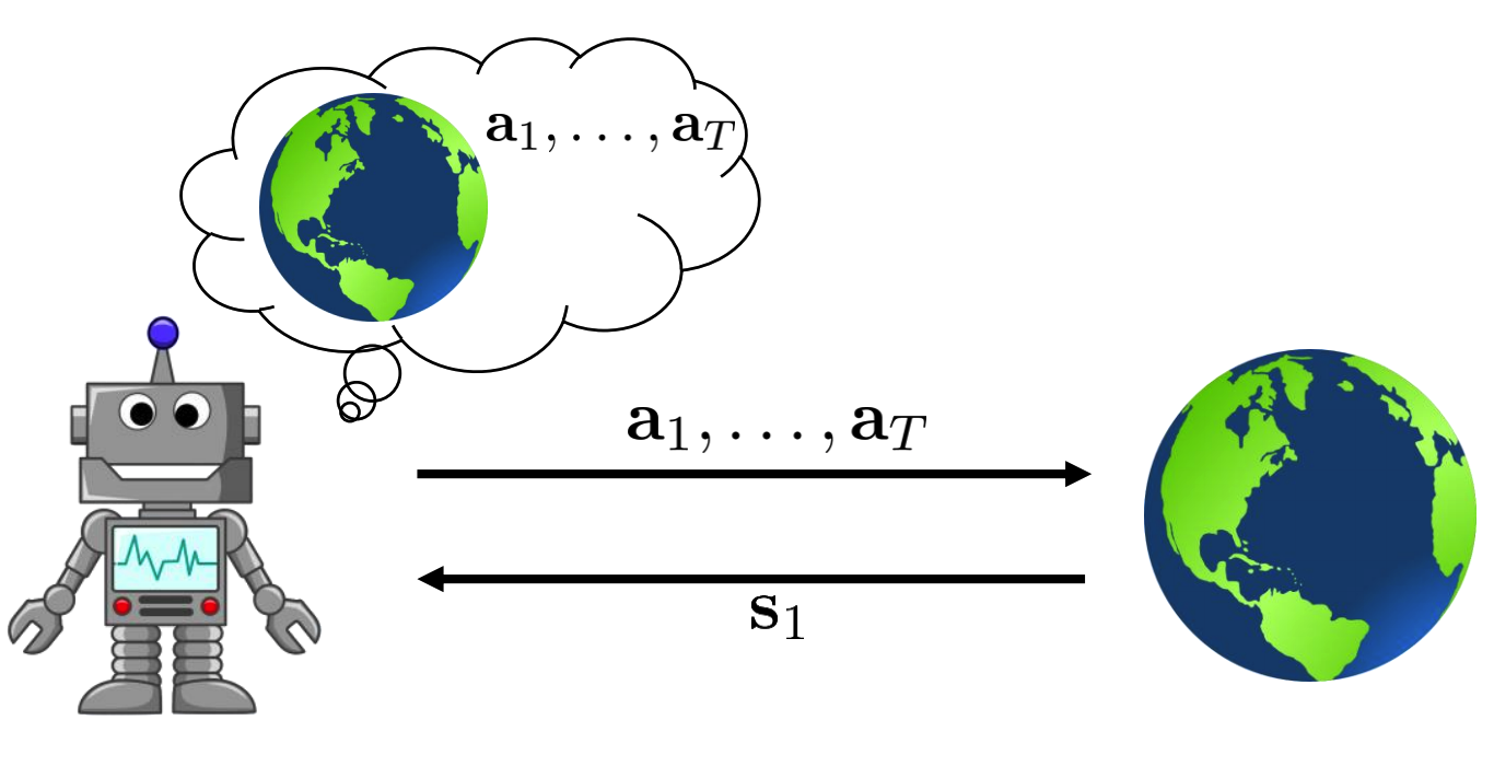
Below we introduce two methods that completely ignore the feedback control and optimize the objective as a blackbox, that is to say, the methods do not even utilize the known dynamics. For simplicity, Let’s write the objective i.e. the expected retrun as \(J(\mathbf{A})\), where \(\mathbf{A} := a_1, a_2, \cdots, a_T\). The goal is to find \(\mathbf{A^*}\) that maximizes this objective.
The first method is called random shooting, which can be explained in one line: randomly sample \(\mathbf{A_1}, \mathbf{A_2}, \cdots, \mathbf{A_N}\) from some distribution (g.e. uniform) and then choose the one that gives the highest \(J(\mathbf{A_i})\) as \(A^*\).
Random shooting seems to be a bad idea, but it actually works well on some low action dimension, short horizon problem. And it’s very easy to implement and parallelize.
However, this is still a overly simple method that completely relies on luck. One method can dramatically improve random shooting method while still maintaining the benefits is called cross-entropy method or CEM. Below the algorithm of CEM:
-
Initialize the actions sequence distribution \(p(\mathbf{A})\)
-
sample \(\mathbf{A_1}, \mathbf{A_2}, \cdots, \mathbf{A_N}\) from \(p(\mathbf{A})\)
-
evaluate \(J(\mathbf{A_1}), J(\mathbf{A_2}), \cdots, J(\mathbf{A_N})\)
-
pick the elites \(\mathbf{A_{i_1}}, \mathbf{A_{i_2}}, \cdots, \mathbf{A_{i_M}}\) with the highest value, where \(M < N\)
-
refit \(p(\mathbf{A})\) to the the elites. Go to 2.
Where setting \(M = 10\%N\) is usually a good choice. The key of CEM is that the action distribution is constantly changing based on the action evaluation. This help the algorithm to find and concentrate the probability mass on areas where actions are more likely to give high value.
Similar to random shooting, CEM is easy to implement and parallelize, while also has harsh dimensionality limits (actions space dimension times the horizon), the exactly limit obviously depends on the problem, but generally these methods cannot go beyond \(60\) dimension, e.g. action dimension is \(5\) and time horizon is \(12\).
2 Monte Carlo Tree Search (MCTS)
In this section we introduce the famous Monte Carlo Tree Search algorithm or MCTS, which has been use in AlphaGO. MTCS is used in cases when the action space is discrete.
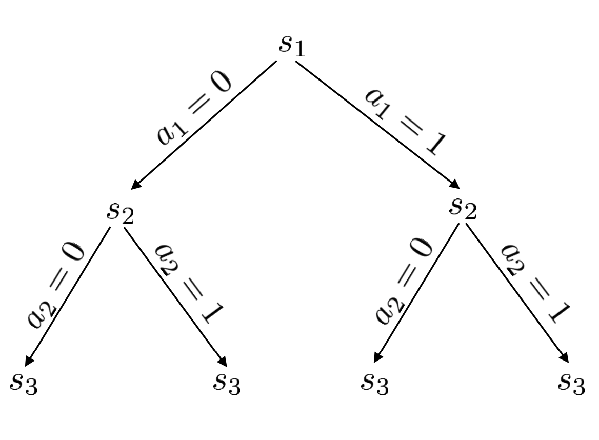
We formulize the problem of planning as a tree search, where the nodes are states and taking different actions leads to the tree branching out to different nodes. Note that the transition can be stochastic and the state space can be contiuous, and in fact, we don’t worry to much about the actual state but only focus on the time step of a state, i.e. \(s_t\) can represent different state at time step \(t\).
Start from the initial state \(s_1\), an naive idea is to just try to take different actions at every state and collect the reward. And after the tree is fully unfold, pick the path that gives the biggest reward.
However, this is prohibitly expensive as the computation complexity is \(O(T^{\lvert\mathcal{A}\rvert})\). MCTS is heuristic method that can approximate the state action value without exactly expand the whole tree. The algorithm is the following:
-
Choose a leaf node \(s_l\) by applying TreePolicy recursively from \(s_1\)
-
Run DefaultPolicy(\(s_{l}\)) and evaluate the the value of \(s_l\)
-
Update all values in tree between \(s_1\) and \(s_l\). While within the computational budget, go back to step 1.
When the algorithm is done, we take the best action starting from \(s_1\).
Now let’s first explain in detail what each steps means, and then we will show an example of how MCTS works.
Step 1. The TreePolicy is basically a node selection strategy. We start from \(s_1\) and recursively apply it to descend through the tree until we find a node that satisfies the strategy and select the node. While there are many strategies, we only introduce one most popular one, namely Upper Confidence Bounds for Trees, or UCT policy. UCT(\(s_t\)) works this way, if \(s_t\) is not fully expanded, i.e. there are possible actions that we haven’t taken, then take that action, if there are multiple actions, just randomly choose one; else, choose a child node \(s_{t+1}\) with the best score Score\((s_{t+1})\), with Score\((s_{t+1})\) is defined as
\[\begin{equation}\label{score} \text{Score}(s_{t+1}) = \frac{Q(s_{t+1})}{N(s_{t+1})} + 2C \sqrt{\frac{2\ln N(s_t)}{N(s_{t+1})}} \end{equation}\]Where \(Q(s_{t+1})\) is the value of the node \(s_{t+1}\), but note that this is not the one that we’ve defined previously in this course, but is an accumulated value - every time we evaluate itself and it’s descedents, we add the value to it. For example, for node \(s_{t+1}\), if we evaluate it self to be \(10\) and later on in the algorithm we evaluate it’s two decendents to be \(5\) and \(11\), then \(Q(s_{t+1}) = 10 + 5 + 11 = 26\). \(N(s_{t+1})\) is the number the node has been visited, in this example, \(N(s_{t+1})\) is \(3\).
Equation \(\ref{score}\) is very intuitive. The first term measure the exact value of the node, the second term measure how often this node has been visited — if \(N(s_t)\) is big, while \(N(s_{t+1})\), that means a lot of visits to \(N(s_t)\) has not pass down to \(N(s_{t+1})\) but other descendents of \(N(s_t)\), and this indicates that we migth want to visit \(N(s_{t+1})\) more often.
Step 2. When we decide to take some action and go to node \(s_l\), we run DefaultPolicy from this state (till it terminates) and collect reward (which we called evaluate the value this node).
Step 3. We add the reward to the value \(Q\) of every node along the path which we follow to get to node \(s_l\). Also update the \(N\) of each node along the path.
Here we put the illustration by Prof. Sergey Levine, Where the illustration starts at 16:50.
3 Linear Quadratic Regulator (LQR)
You might notice that methods introduced in previous two sections actually do not require a known dynamics. In this section, we will finally introduce methods that do require and utilize a known dynamics. since the methods in this section are mostly studied in the optimal control community, we will follow the their notation and denote action as \(u_t\), state as \(x_t\), dynamics as \(x_{t+1} = f(x_t, u_t)\) or \(x_{t+1}\sim p(x_{t+1}\mid x_t, u_t)\), and cost as \(c(x_t, u_t)\). This is the first time the term “cost” appears in this series, but it’s really just the opposite of reward, where reward measures how good an action state pair is, and cost measures how bad an action state pair is. Note that different from the classic RL setting, in addition to the dynamics, we also assume the cost function is known.
Similar to policy gradient methods, we aim at directly minimizing the sum of cost:
\[\begin{align} &\min_{u_1,\cdots, u_T}\sum_{t=1}^{T}c(x_t, u_t) \\ &\text{s.t.} x_{t+1} = f(x_t, u_t) \end{align}\]We can actually incorporate the constraint into the objective and make it an uncontraint optimization problem:
\[\begin{align}\label{obj} &\min_{u_1,\cdots, u_T}\, c(x_1, u_1) + c(f(x_1,u_1), u_2) + \cdots + c(f(f(\cdots)\cdots),u_T) \end{align}\]Linear Quadratic Regulator or LQR further simpifies this problem by assume a linear dynamics and quadratic cost:
\[\begin{equation} \begin{aligned} & f(x_t, u_t) = F_t \begin{bmatrix} x_t \\ u_t \end{bmatrix} + f_t \\ & c(x_t, u_t) = \frac12 \begin{bmatrix} x_t \\ u_t \end{bmatrix}^T C_t \begin{bmatrix} x_t \\ u_t \end{bmatrix} + \begin{bmatrix} x_t \\ u_t \end{bmatrix}^T c_t \end{aligned} \end{equation}\]Note that \(F_t, f_t, C_t, c_t\) are all known quantities.
To solve LQR, the simplest method is just take the derivative of the objective w.r.t. actions and set them to \(0\). But this is numerically very unstable because the sensitivities of actions at different time step to the cost is very different, for example, the first action is in every term of the objective and has a huge effect on the total cost, while the last action has a very small effect.
We introduce a stable iterative method to solve LQR. We start from the last action \(u_T\), since it doesn’t affect previous states and also has no affect on future states (there is no future state!). Treat all terms that are not effected by \(u_T\) as constant, we can write the cost as
\[\begin{equation} \begin{aligned} Q(x_T, u_T) = \text{const.} + \frac12 \begin{bmatrix} x_T \\ u_T \end{bmatrix}^T C_T \begin{bmatrix} x_T \\ u_T \end{bmatrix} + \begin{bmatrix} x_T \\ u_T \end{bmatrix}^T c_T \end{aligned} \end{equation}\]take the derivative
\[\begin{align*} &\nabla_{u_T}Q(x_T, u_T) = C_{u_T, x_T}x_T + C_{u_T, x_T}u_T + c_{u_T}^T = 0 \\ &\Rightarrow u_T = -C_{u_T, u_T}^{-1}(C_{u_T, x_T}x_T + c_{u_T}) \end{align*}\]where
\[\begin{equation} \begin{aligned} C_T = \begin{bmatrix} C_{x_T, x_T} & C_{x_T, u_T}\\ C_{u_T, x_T} & C_{u_T, u_T} \end{bmatrix} \quad c_T = \begin{bmatrix} c_{x_T} \\ c_{u_T} \end{bmatrix} \end{aligned} \end{equation}\]To better see the pattern (useful for later derivation), we denote
\[\begin{align*} &K_T = -C_{u_T, u_t}^{-1}C_{u_T, x_t} \\ &k_T = - C_{u_T, u_T}^{-1}c_{u_T} \end{align*}\]and write \(u_T\) as
\[\begin{equation}\label{xt} u_T = K_Tx_T + k_T \end{equation}\]This equation shows that the optimal \(u_T\) is a linear function of \(x_T\).
Our goal is to represent \(u_t\)’s using \(x_t\)’s and then once we have the first state \(x_1\), we can get \(u_1\), and then via the dynamics we have \(x_2\) and then \(u_2\) etc. This way, we can get all the actions (and states).
Now let’s try to represent optimal \(u_{T-1}\) using \(x_{T-1}\). Note that \(u_{T-1}\) can only affect \(x_T, u_T\), and thus we can treat all terms that are not effected by \(u_{T-1}\) as constant and write the objective as
\[\begin{equation} \begin{aligned} &Q(x_{T-1}, u_{T-1}) \\ &= \text{const.}+ \frac12 \begin{bmatrix} x_{T-1} \\ u_{T-1} \end{bmatrix}^T C_{T-1} \begin{bmatrix} x_{T-1} \\ u_{T-1} \end{bmatrix} + \begin{bmatrix} x_{T-1} \\ u_{T-1} \end{bmatrix}^T c_{T-1} \\ +& \frac12 \begin{bmatrix} x_T \\ K_Tx_T + k_T \end{bmatrix}^T C_T \begin{bmatrix} x_T \\ K_Tx_T + k_T \end{bmatrix} + \begin{bmatrix} x_T \\ K_Tx_T + k_T \end{bmatrix}^T c_T \\ &=\text{const.}+\frac12 \begin{bmatrix} x_{T-1} \\ u_{T-1} \end{bmatrix}^T C_{T-1} \begin{bmatrix} x_{T-1} \\ u_{T-1} \end{bmatrix} + \begin{bmatrix} x_{T-1} \\ u_{T-1} \end{bmatrix}^T c_{T-1} + \frac12 x_T^TV_Tx_T + x^T_T v_T \end{aligned} \end{equation}\]Where \(V_T, v_T\) are terms that depends on \(C_T, c_T\) only. We can see that this is again a sum of linear and quadratic terms of \(x_{T-1}, u_{T-1}\).
We can take the derivative of it w.r.t. \(u_{T-1}\) and set it to \(0\). We will get:
\[\begin{equation}\label{xt-1} u_{T-1} = K_{T-1}x_{T-1} + k_{T-1} \end{equation}\]Where \(K_{T-1}\) and \(k_{T-1}\) are functions of \(F_{T-1}, f_{t-1}, C_{T-1}, c_{T-1}. V_T, v_T\), the expression is a bit hairy, but the important thing to known that \(K_{T-1}\) and \(k_{T-1}\) are known quantities.
Therefore we show that we can always represent \(u_t\) as a linear function of \(x_t\).
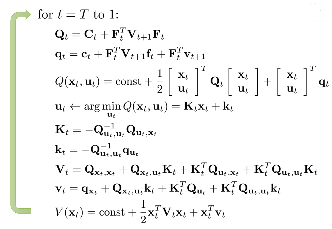
The full algorithm contains first starting from time step \(T\) and go backward to represent \(u_t\) using \(x_t\), and then run forward from time step \(1\) to get action state and action at every time step.
Concretly, the backward iteration is
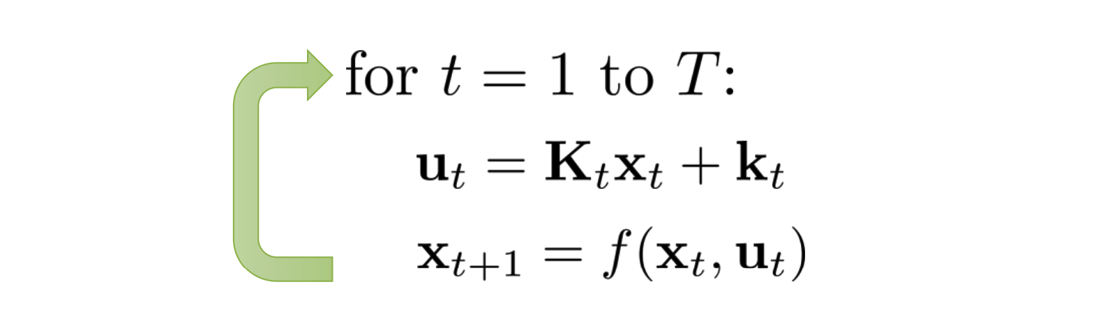
And the forward iteration is
4 LQR for Stochastic and Nonlinear Systems
4.1 Guassian Dynamics
When the dynamics is stochastic, we want to minimize the expected cost
\[\begin{equation}\label{sto} \min_{u_1, \cdots, u_T}\mathbb{E}\sum_{t=1}^{T}c(x_t, u_t) \end{equation}\]Where the expectation is taken w.r.t dynamics \(p(x_{t+1}\mid x_t, u_t)\).
Here we briefly introduce applying LQR in a special case of stochastic dynamics — Guassian linear dynamics
\[\begin{align*} p(x_{t+1}\mid x_t, u_t) = \mathcal{N}( F_t \begin{bmatrix} x_t \\ u_t \end{bmatrix} + f_t, \Sigma_t ) \end{align*}\]It turns out that if the cost is still quadratic in state and action, the objective in equation \(\ref{sto}\) can be solved analytically and we can apply the same iterative procedure and actually get the same solution \(u_t = K_t x_t + k_t\). Details are left to the readers.
4.2 Iterative LQR (iLQR) for Nonlinear Systems
Now we get rid of the assumption that the dynamics is linear and cost is quadratic.
We can use first Taylor expansion to approximate the dynamics as
\[\begin{align} f(x_t, u_t) \approx f(\hat{x}_t, \hat{u}_t) + \nabla_{x_t, u_t}f(\hat{x}_t, \hat{u}_t) \begin{bmatrix} x_t - \hat{x}_t \\ u_t - \hat{u}_t \end{bmatrix} \end{align}\]Use second order Taylor expansion to approximate cost as
\[\begin{align} c(x_t, u_t) \approx c(\hat{x}_t, \hat{u}_t) + \nabla_{x_t, u_t}c(\hat{x}_t, \hat{u}_t) \begin{bmatrix} x_t - \hat{x}_t \\ u_t - \hat{u}_t \end{bmatrix} \\ + \frac12 \begin{bmatrix} x_t - \hat{x}_t \\ u_t - \hat{u}_t \end{bmatrix}^T \nabla_{x_t, u_t}^2 c(\hat{x}_t, \hat{u}_t) \begin{bmatrix} x_t - \hat{x}_t \\ u_t - \hat{u}_t \end{bmatrix} \end{align}\]Denote
\[\begin{align} \delta x_t = x_t - \hat{x}_t \\ \delta u_t = u_t - \hat{u}_t \\ f_t = f(\hat{x}_t, \hat{u}_t) \\ F_t = \nabla_{x_t, u_t}f(\hat{x}_t, \hat{u}_t) \\ c_t = \nabla_{x_t, u_t}c(\hat{x}_t, \hat{u}_t) \\ C_t = \nabla_{x_t, u_t}^2 c(\hat{x}_t, \hat{u}_t) \end{align}\]No need to worry about the constant term \(c(\hat{x}_t, \hat{u}_t)\) in cost approximation, as it will disappear when we take the derivative, i.e. it will not affect the solution.
We can first randomly pick sequence of actions as \(\hat{u}_t\)’s and then get the states \(\hat{x}_t\) based on the true dynamics. Then, run backward and forward LQR algorithm on
\[\begin{equation} \begin{aligned} & f(\delta x_t, \delta u_t) = F_t \begin{bmatrix} \delta x_t \\ \delta u_t \end{bmatrix} + f_t \\ & c(\delta x_t, \delta u_t) = \frac12 \begin{bmatrix} \delta x_t \\ \delta u_t \end{bmatrix}^T C_t \begin{bmatrix} \delta x_t \\ \delta u_t \end{bmatrix} + \begin{bmatrix} \delta x_t \\ \delta u_t \end{bmatrix}^T c_t \end{aligned} \end{equation}\]which gives \(\delta x_t, \delta u_t\), add them by \(c(\hat{x}_t, \hat{u}_t)\) and we get the \(x_t\)’s and \(u_t\)’s, we then denote them as \(\hat{x}_t, \hat{u}_t\), and repeat the process. Put it in one place, the algorithm is the following:
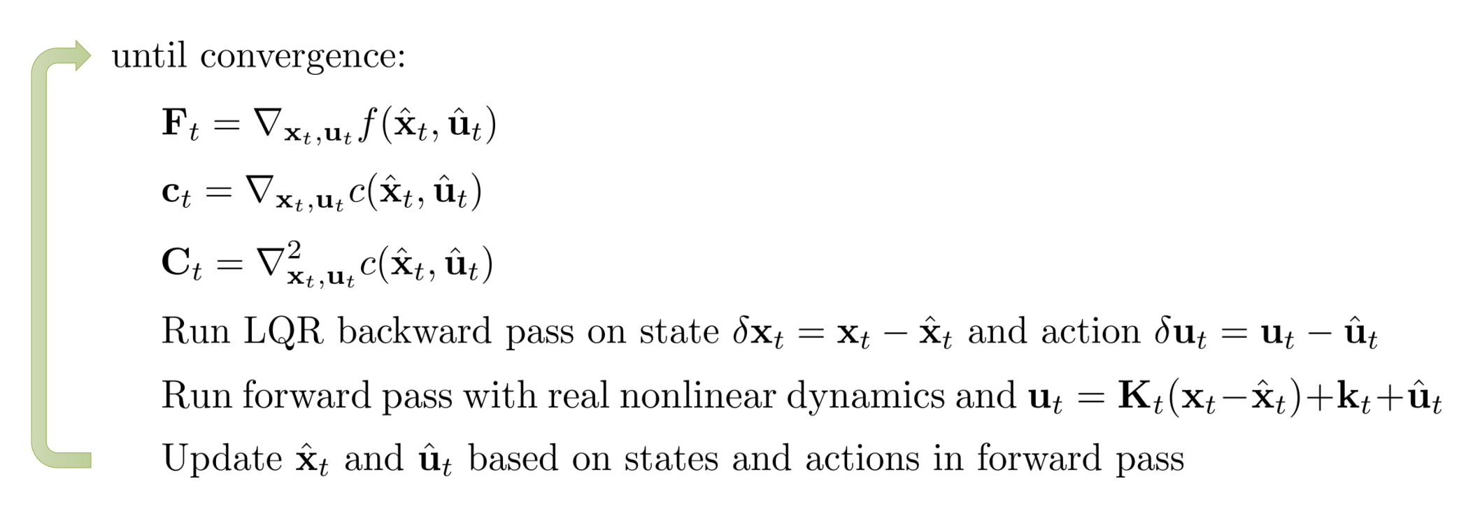
Note that in the forward pass of LQR, we use the true dynamics rather than the quadratic approximation, to get the states. When \(\hat{x}_t, \hat{u}_t\)’s are very close to \(x_t, u_t\) newly obtained the current LQR forward iteration, we say the algorithm has converged.
This algorithm is very similar to Newton’s method, and in fact, the only difference is that Newton’s method will approximate dynamics using second order Taylor expension.
Since we are using approximations, too big a step in the update may lead to worse result due too the approximations being inaccurate. To rememdy this, when runnig the forward pass to get \(u_t\), we introduce a parameter \(\alpha\), and change the update rule to be
\[\begin{equation} u_t = K_t(x_t - \hat{x}_t) + \alpha k_t + \hat{u}_t \end{equation}\]\(\alpha\) controls the step size in the update (how much \(u_t\) will deviate from \(\hat{u}_t\)). And we can perform a search over \(\alpha\), until we see improvements on the cost.