
Deep RL 11 Model-Based Policy Learning
In this section, we study how to learn policies utilize the known (learned) dynamics. Why do we need to learn a policy? What’s wrong with MPC in the previous lecture? The answer is that MPC is still an open loop control methods, even though the replanning machanism provides some amount of closed-loop capability, but the planning procedure still is unable to reason under the fact that more information will be revealed in the future and we can act based on that information. This is obviously suboptimal in the stochastic dynamics setting.
On the other hand, if we have an explicit policy, we can make decision at each time step based on the state at that time step, and therefore no need to plan the whole action sequence all in one go. This is closed-loop planning and it’s more desirable in the stochastic dynamics setting.
1 Learn Policy by Backprop Through Time (BPTT)
Suppose we have learned dynamics \(s_{t+1} = f(s_t, a_t)\) and reward function \(r(s_t, a_t)\), and want to learn optimal policy \(a_t = \pi_{\theta}(s_t)\). (Here is use deterministic dynamics and policy to make a point. The point also applies to stochastic dynamics, but the derivation is slightly more involved and will be introduced in the future; Also I drop the parameters notation in the dynamics and reward function for simplicity). Same as policy gradient, our goal will be:
\[\begin{align} \theta^* = \text{argmax}_{\theta} \mathbb{E}_{\tau\sim p(\tau)}\sum_t r(s_t, a_t) \end{align}\]Since we have dynamics and reward function, we can write the objective as
\[\begin{align} \mathbb{E}_{\tau\sim p(\tau)}\sum_t r(s_t, a_t) = \sum_t r(f(s_{t-1}, a_{t-1}), \pi_{\theta}(f(s_{t-1}, a_{t-1}))), \text{ where } s_{t-1} = f(s_{t-2}, a_{t-2}) \end{align}\]Very similar to shooting methods, the objective is defined recursively, which lead to high sensitivity to the first actions and lead to poor numerical stability. However, for shooting methods, if we define the process as LQR, we can use a dynamical programming to solve it in a very stable fashion. Unfortunately, unlike LQR, since the the parameters of the policy couple all time steps, we cannot solve by dynamical programming (i.e. can’t calculate the best policy parameter for the last time step and solve for the policy parameters for second to last time step and so on).
What we can use is backpropagation:
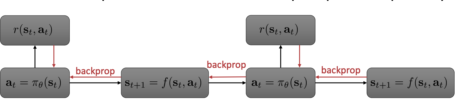
If you are familiar with recurrent neural network, we might realize that the kind of backprop shown above is the so called Backpropagation Through Time or BPTT, which is usually used on recurrent neural nets like LSTM. BPTT famously has the vanishing or exploding gradients issue, because all the jacobians of different time steps get multiplied together. This issue can only get worse in policy learning, because in sequence deep learning, we can choose architectures like LSTM that has good gradient behavior, but in model-based RL, the dynamics has to fit to the data and we don’t have control over the gradient behavior.
In the next two sections, we will introduce two popular ways to model-based RL. The first way is a bit controvesal, it does model-free optimization (policy gradient, actor-critic, Q-learning etc.) and use model to only generate sythetic data. Despite looking weird backwards, this idea can work very well in pratice; the second way is to use simple local models and local policies, which can be solved using stable algorithms.
2 Model-Free Optimization with a Model
Reinforcement learning is about getting better by interacting with the world, and the interacting, try-and-error process can be time consuming (even in a simulator sometimes). If we have a mathematical model that represent how the world works, then we can effortlessly generate data (transitions) from it for model-free algorithms to get better. However, it’s impossible to have a comprehansive mathematical model of the world, or even of the environment we want to run our RL algorithms. Nevertheless, a learned dynamics is a representation of the environment and we can use it to generate data.
The general idea is to use the learned dynamics to provide more training data for model-free algorithms, it does it by generate model-based rollouts from real world states.
The general algorithm is the following:
- run some policy in the environment to collect data \(\mathcal{B}\)
- sample minibatch \({(s, a, r, s')}\) from \(\mathcal{B}\) uniformly
- use \({(s, a, r, s')}\) to update model and reward function
- sample minibatch {(s)} from \(\mathcal{B}\)
- for each \(s\), perform model-based k step rollout with neural net policy \(\pi_{\theta}\) or policy indiced from Q-learning , get transitions \({(s, a, r, s')}\)
- use the transitions for policy gradient update or updating Q-function. Go to step 4 for a few more times (inner loop); Go to step 1 (outer loop).
There are a few things to be cleared. Above algorithm is very general and explicitly considers both policy gradient and Q-learning, this will affect what we actually do in step 1, 5, and 6. If we use policy gradient, in step 1 and step 5, we can run the learned policy, and in step 6, we run policy gradient update; if we use Q-learning, then in step 1 and step 5, we run policy indiced by the learned Q-function, e.g. \(\epsilon\)-greedy policy. And in step 6 we update the Q-function by taking the gradient of temporal difference.
Model-based rollout step k is an very important hyperparameter, since we completely reply on \(f_{\phi}(s_t, a_t)\) during model-based rollout, the discrepancy between \(f_{\phi}(s_t, a_t)\) and the ground truth dynamics can result in a distribution shift problem, i.e. the expectation in the objective we are optimizing is over a distribution that is very different from the true distribution. We’ve encounter this issue several times (e.g. imitation learning, TRPO etc.). We know that if there is a discrepancy between fitted dynamics and true dynamics, the error between true objective and the objective we optimizes grow linearly with the length of rollout. Therefore, we don’t want the length of model-based rollout to be too long; on the other hand, too short a rollout provide little learning signal, which is undesirable for policy update or Q-function update. Therefore, we need to choose an appropriate k for the algorithm.
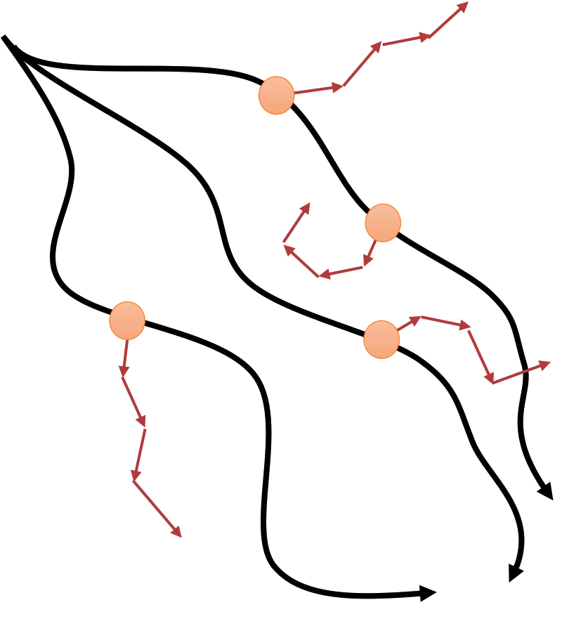
Since for every model-based rollout, the initial state is sampled from real world data, this algorithm can be intuitively understand as imagining different possibilities starting from real world situations:
Here we give one instatiation of the general algorithm introduced above, which combines model-based RL with policy gradient methods. The algorithm is called Model-Based Policy Optimization or MBPO Janner et al. 19’:
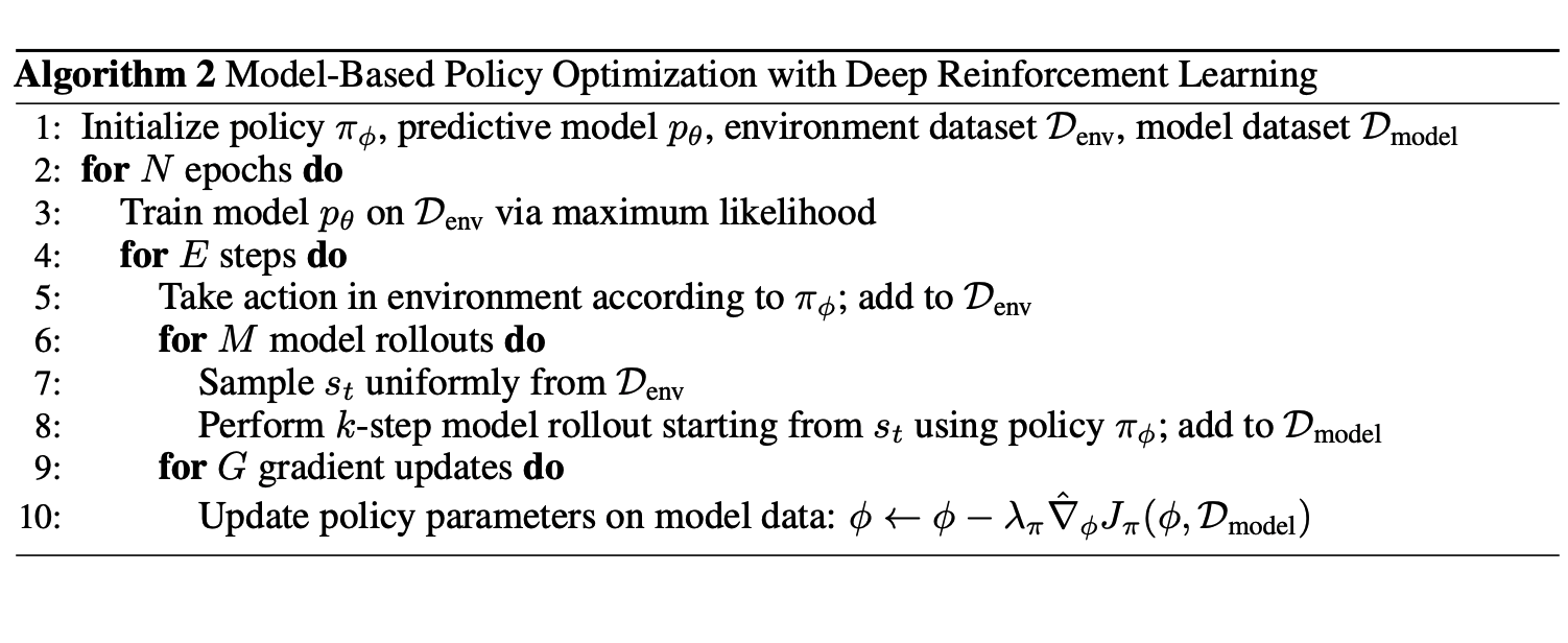
For instatiation with Q-learning, see Gu et al. 16’ and Feinberg et al 18’.
3 Use Simpler Policies and Models
3.1 LQR with Learned Models
A local model is a model that is valid only in the neighborhood of one or some trajectories. Previously, we learned (i)LQR, which assumes linear dynamics (approximates dynamics by a linear function), which could be too simple for most scenarios, but it might be a good assumption locally, i.e. for one or a few very close trajectories, we can assume a linear dynamics. Suppose we are given these trajectories, we want fit a linear dynamics to it by linear regression at each time step, and then perform (i)LQR to get actions and execute these actions in the environment, we can get new trajectories, and we can again fit a linear dynamics to these trajectories, and then run (i)LQR and execute the planned actions……
The procedure looks like the following:
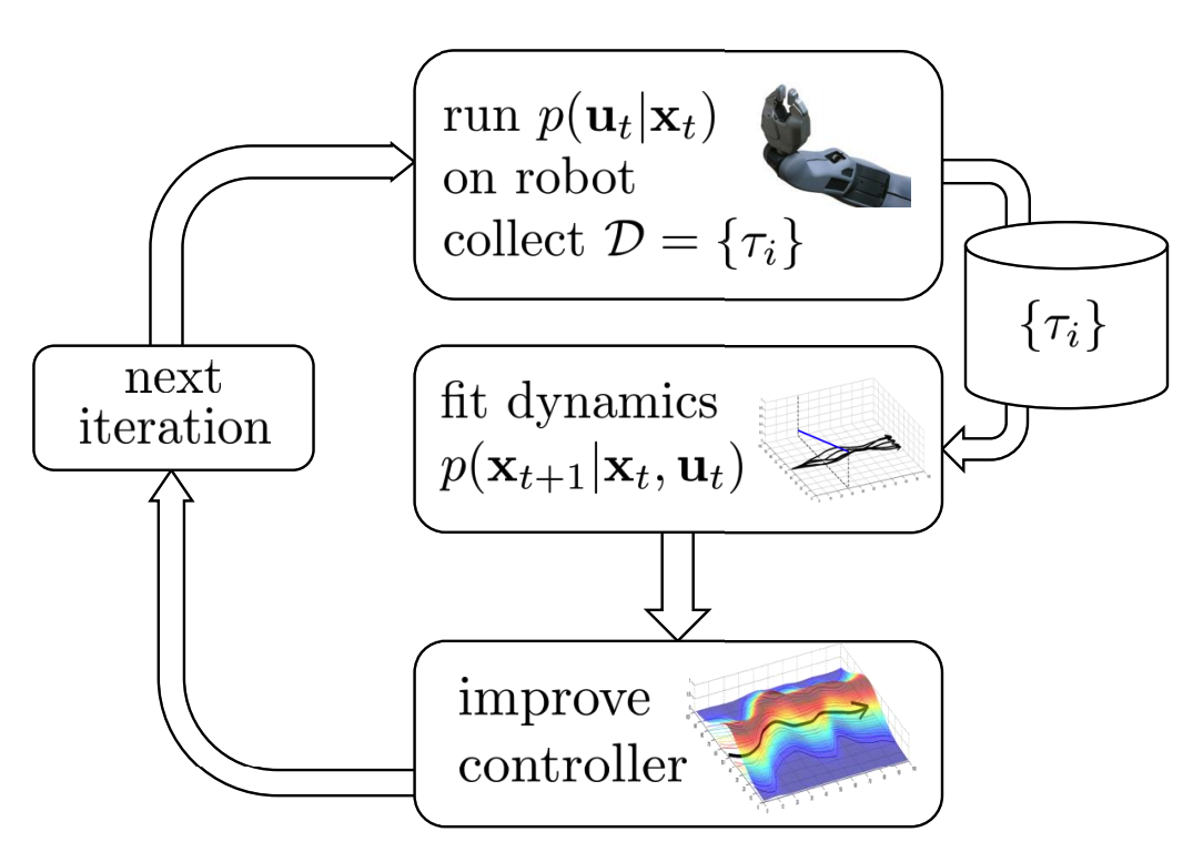
Where the local linear dynamics is defined as
\[p(x_{t+1}\mid x_t, u_t) = \mathcal{N}(A_t x_t + B_t u_t + c_t, \Sigma)\]Where \(A_t, B_t, c_t\) are to be fitted using trajectories \(\{ \tau_i \}\). \(\Sigma\) can be tuned as a hyperparameter or also be estimated from data.
The policy is defined as
\[p(u_t\mid x_t) = \mathcal{N}(K_t (x_t - \hat{x_t}) + k_t + \hat{u_t}, \Sigma_t)\]Note that this correspond to iLQR, i.e. \(K_t, k_t\) are calculated from the fitted dynamics and \(\hat{x_t}, \hat{u_t}\) are the actual states and actions in the trajectories \(\{ \tau_i \}\). \(\Sigma_t\) is set to be \(Q_{u_t, u_t}^{-1}\), which is also intermediate result of running iLQR. Intuitively, \(Q_{u_t, u_t}\) is gradient of the cost to go w.r.t. the action. If the gradient is low, that means the total reward doesn’t depend very strongly on the action, which means many different actions may lead to similar reward, then it’s a good idea to test out different actions, so we want the variance of \(p(u_t\mid x_t)\) to be high, and vice versa. Setting \(\Sigma_t\) to be \(Q_{u_t, u_t}^{-1}\) gives us such property.
One more thing to notice is that since the fitted dynamics is only valid locally, if the action we take lead to very different state distribution then the subsequent actions planned might be very bad and lead to even worse result. Therefore, we need to make sure the new trajectory distribution is close enough to the old distribution. This can be inforced by using again using KL divergence:
\[D_{\text{KL}}(p_{\text{new}}(\tau) \lvert p_{\text{old}}(\tau))\]For details about how this is implemented, please see Sergey and Abbeel 14’.
3.2 Guided Policy Search
If we have a bunch of local policies e.g. \(\{\pi_{\text{LQR, i}}\}_{i}\), which are derived from local models (e.g. LQR models), we can distill the knowledge of these local policies to get a global policy by supervised learning.
The idea above can be view as a special case of a more general framework is known as knowledge distillation (Hinton et al. 15’). Here we have a bunch of weak policies (local policies) and we can ensemble them to get a strong policy, but rather than directly using the ensemble, we distill knowledge from this ensemble to get one global neural network policy \(\pi_{\theta}\).We train the neural network using the trajectories we used for training LQR parameters and policies, except that instead of directly train the neural net policy to output the one actual action sequence at each time step, we train the neural net to predict probability of each action given the state.
In order for the algorithm to work better, we want the LQR policy \(\{\pi_{\text{LQR, i}}\}_{i}\) to be close to the neural net policy \(\pi_{\theta}\). We use KL divergence to inforce that, and it can be implemented as modifying the cost function of LQR.
The algorithm sketch is the following:
- Optimize each local policy \(\pi_{\text{LQR, i}}\) on initial state \(x_{0,i}\) w.r.t \(\tilde{c}_{k,i}(x_t, u_t)\)
- use samples from step one one to train \(\pi_{\theta}\) to minic each \(\pi_{\text{LQR, i}}\)
- update cost function \(\tilde{c}_{k+1,i}(x_t, u_t) = c(x_t, u_t) + \lambda_{k+1, i}\log \pi_{\theta}(u_t\mid x_t)\). Go to step 1.
Where \(k\) index is number of the step in the algorithm and \(i\) index different LQR models which is instantiated by starting from different initial state. Step 3 is for making local policies and the global policy close to each other in terms of KL divergence and \(\lambda_{k+1, i}\) is the Lagrangian multiplier. This is just a sketch of the algorithm, and for details, please checkout the original paper by Levine and Finn et al. 16’.
Similar approach can also be extended to multitask transfer scenario:
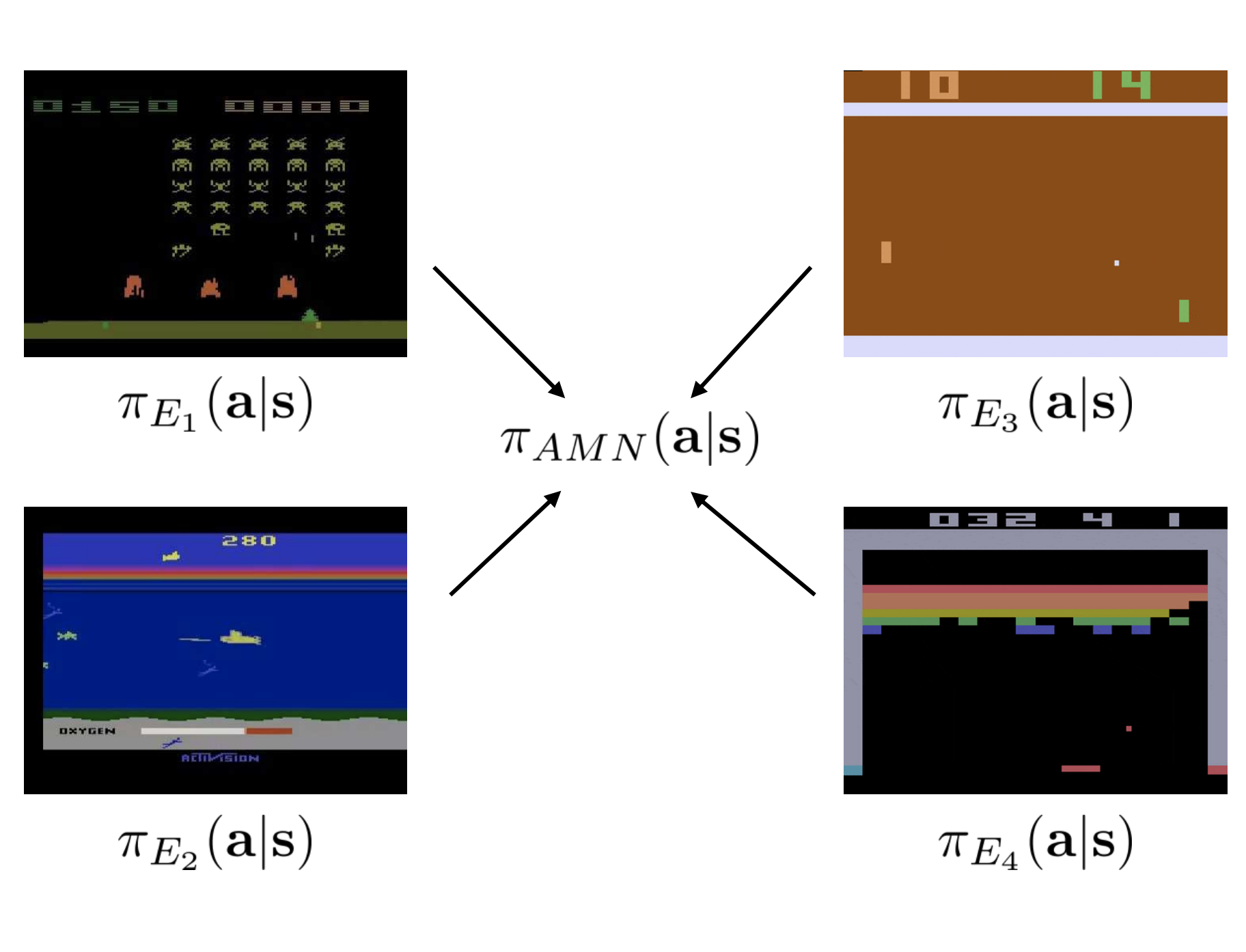
Where the loss function for training the global policy is
\[\mathcal{L}^i = \sum_{a\in \mathcal{A}_{E_i}} \pi_{E_i(a\mid s)}\log \pi_{\theta}(a\mid s)\]For deteils, please see Parisotto et al. 16’.