Deep RL 8 Advanced Policy Gradient

At the end of previous lecture, we talked about the issues with Q-learning, one of them is that it’s not directly optimizing the expected return and it can take a long time before the return starts to improve. On the other hand, policy gradient methods are direclty optimizing the expected return, although we cannot guarantee that the return will improve every gardient update. At the same time, we know that classic policy iteration can improve the expected return at each iteration, but this method cannot be applied to large scale problems.

In this section, we derive stable policy gradient methods, by firstly framing them as policy iteration.

1 Policy Gradient as Policy Iteration

Let’s write down the difference between expected return under previous policy \(q\) and under new (updated) policy \(\pi_{\theta'}\):

\[\begin{align} &J(\theta') - J(\theta)\\ &= \mathbb{E}_{\tau \sim p_{\theta'}(\tau)}\left[ \sum_t \gamma^tr(s_t, a_t) \right] - \mathbb{E}_{\tau \sim p_{\theta}(\tau)}\left[ \sum_t \gamma^tr(s_t, a_t) \right] \\ &= \mathbb{E}_{\tau \sim p_{\theta'}(\tau)}\left[ \sum_t \gamma^tr(s_t, a_t) \right] - \mathbb{E}_{s_0 \sim p(s_0)}\left[ V^{q}(s_0) \right] \\ &= \mathbb{E}_{\tau \sim p_{\theta'}(\tau)}\left[ \sum_t \gamma^tr(s_t, a_t) \right] - \mathbb{E}_{\tau \sim p_{\theta'}(\tau)}\left[ V^{q}(s_0) \right] \\ &= \mathbb{E}_{\tau \sim p_{\theta'}(\tau)}\left[ \sum_t \gamma^tr(s_t, a_t) \right] - \mathbb{E}_{\tau \sim p_{\theta'}(\tau)}\left[ V^{q}(s_0) + \sum_{t=1}^{\infty}\gamma^{t}V^{q}(s_{t}) - \sum_{t=1}^{\infty}\gamma^{t}V^{q}(s_{t}) \right] \\ &= \mathbb{E}_{\tau \sim p_{\theta'}(\tau)}\left[ \sum_t \gamma^tr(s_t, a_t) \right] + \mathbb{E}_{\tau \sim p_{\theta'}(\tau)}\left[ \sum_t\gamma^{t}(\gamma V(s_{t+1}) - V^{q}(s_{t})) \right] \\ &= \mathbb{E}_{\tau \sim p_{\theta'}(\tau)}\left[ \sum_t \gamma^t(r(s_t, a_t) + \gamma V(s_{t+1}) - V^{q}(s_{t})) \right] \\ &= \mathbb{E}_{\tau \sim p_{\theta'}(\tau)}\left[ \sum_t \gamma^t A^{\pi_{\theta}}(s_t, a_t) \right] \end{align}\]

Here we have proved an intersting equality:

\[\begin{equation}\label{diff} J(\theta') - J(\theta) = \mathbb{E}_{\tau \sim p_{\theta'}(\tau)}\left[ \sum_t \gamma^t A^{\pi_{\theta}}(s_t, a_t) \right] \end{equation}\]

The difference of expected return equals to the expected value of the advantage of the previous policy \(q\) under the trajectory distribution of the new policy \(\pi_{\theta'}\).

Note that we haven’t done any policy gradient specific operation, so this equality is universal. We can use this to understand why policy iteration improve the expected return at every iteration i.e. \(J(\theta') - J(\theta) \geq 0\): in policy iteration, the policy is deterministic and updated as \(\pi'(s) = \text{argmax}_a A^{\pi}(s_t, a_t)\). Therefore when the \(s_t, a_t\) are from the new policy \(\pi'\), we always have \(A^{\pi_{\theta}}(s_t, a_t) \geq 0\), and thus \(J(\theta') - J(\theta) \geq 0\).

Now let’s consider how to have this monotonic improvement in expected return in policy gradient methods. Well, this cannot be guaranteed theoretically because we need to introduce some approximation in order to derive a policy gradient algorithm from equation \(\ref{diff}\). Nevertheless, the resulting method — TRPO — is the first stable RL algorithm in that during training the return will improve gradually (whereas another popular methods at the time — DQN — is very unstable).

2 Trust Region Policy Optimization (TRPO) Setup

As a policy gradient method, TRPO aims at directly maximizing equation \(\ref{diff}\), but this cannot be done because the trajectory distribution is under the new policy \(\pi_{\theta'}\) while the sample trajectories that we have can onlu come from the previous policy \(q\).

This might reminds you on importance sampling that we used for deriving off-policy policy gradient. Yes, we will rewrite equation \(\ref{diff}\) using importance sampling:

\[\begin{align} &J(\theta') - J(\theta) \\ &= \mathbb{E}_{\tau \sim p_{\theta'}(\tau)}\left[ \sum_t \gamma^t A^{\pi_{\theta}}(s_t, a_t) \right] \\ &= \sum_t\mathbb{E}_{s_t\sim p_{\theta'}(s_t)}\left[ \mathbb{E}_{a_t \sim \pi_{\theta'}} \gamma^t A^{\pi_{\theta}}(s_t, a_t)\right]\\ &= \sum_t\mathbb{E}_{s_t\sim p_{\theta'}(s_t)}\left[ \mathbb{E}_{a_t \sim q} \frac{\pi_{\theta'}(a_t\mid s_t)}{q(a_t\mid s_t)}\gamma^t A^{\pi_{\theta}}(s_t, a_t)\right] \label{diff_importance} \end{align}\]

However, even though we don’t need to sample from \(p_{\theta'}(\tau)\) now, \(p_{\theta'}(s_t)\) is still impossible. A natural question is, can we just use \(p_{\theta}(s_t)\)? I.e. approximating the equation above by

\[\begin{align} &\approx \sum_t\mathbb{E}_{s_t\sim p_{\theta}(s_t)}\left[ \mathbb{E}_{a_t \sim q} \frac{\pi_{\theta'}(a_t\mid s_t)}{q(a_t\mid s_t)}\gamma^t A^{\pi_{\theta}}(s_t, a_t)\right] \\ &= \mathbb{E}_{\tau \sim p_{\theta}(\tau)}\left[ \sum_t \frac{\pi_{\theta'}(a_t\mid s_t)}{q(a_t\mid s_t)}\gamma^t A^{\pi_{\theta}}(s_t, a_t) \right] \label{final} \end{align}\]

Eqaution \(\ref{final}\) will lead to almost the same gradient as the off-policy policy gradient, but with reward \(r(s_t, a_t)\) begin replaced by advantage \(A^{\pi_{\theta}}(s_t, a_t)\). And you might remember that we also used \(p_{\theta}(s_t)\) to approaximate \(p_{\theta'}(s_t)\) and briefly mentioned that this approximation error “is bounded when the gap between \(q\) and \(\pi_{\theta'}\) are not too big”.

Now let’s try to quantitative give the gap between \(q\) and \(\pi_{\theta'}\). The first quantitative gap actually has been introduced in lecture 2 when we introduce the error bound on DAgger for imitation learning — we define \(\pi_{\theta'}\) is close to \(\pi_{\theta}\) if

\[\begin{equation}\label{cond1}\left| \pi_{\theta'}(a_t\mid s_t) - \pi(a_t\mid s_t)\right|< \epsilon, \forall s_t\end{equation}\]

This will give

\[\begin{align*} &\left| p_{\theta'}(s_t) - p_{\theta}(s_t) \right|\\ &= \left| (1-\epsilon)^tp_{\theta}(s_t) + (1-(1-\epsilon)^t)p_{\text{mistake}}(s_t) - p_{\theta}(s_t) \right|\\ &= (1-(1-\epsilon)^t)\left| p_{\text{mistake}}(s_t) - p_{\theta}(s_t) \right|\\ &\leq 2(1-(1-\epsilon)^t)\\ &\leq 2\epsilon t \end{align*}\]

This is very similar to the derivation we have for DAgger, and if there is anything that is unclear to you, please see lecture 2 section 3.2.

Now let’s reveal what \(\lvert p_{\theta'}(s_t) - p_{\theta}(s_t) \rvert \leq 2\epsilon t\) can bring us:

Since

\[\begin{align*} &\mathbb{E}_{p_{\theta'}(s_t)}\left[ f(s_t) \right]\\ &= \sum_{s_t}p_{\theta'}(s_t)f(s_t) \\ &\geq \sum_{s_t}p_{\theta}(s_t)f(s_t) - \left|p_{\theta'}(s_t) - p_{\theta}(s_t)\right|\max_{s_t}f(s_t)\\ &\geq \sum_{s_t}p_{\theta}(s_t)f(s_t) - 2\epsilon t \max_{s_t}f(s_t) \end{align*}\]

Therefore, we have

\[\begin{align} &\sum_t\mathbb{E}_{s_t\sim p_{\theta'}(s_t)}\left[ \mathbb{E}_{a_t \sim q} \frac{\pi_{\theta'}(a_t\mid s_t)}{q(a_t\mid s_t)}\gamma^t A^{\pi_{\theta}}(s_t, a_t)\right] \\ &\geq \sum_t\mathbb{E}_{s_t\sim p_{\theta}(s_t)}\left[ \mathbb{E}_{a_t \sim q} \frac{\pi_{\theta'}(a_t\mid s_t)}{q(a_t\mid s_t)}\gamma^t A^{\pi_{\theta}}(s_t, a_t)\right] - \sum_t 2\epsilon t C \\ &\geq \sum_t\mathbb{E}_{s_t\sim p_{\theta}(s_t)}\left[ \mathbb{E}_{a_t \sim q} \frac{\pi_{\theta'}(a_t\mid s_t)}{q(a_t\mid s_t)}\gamma^t A^{\pi_{\theta}}(s_t, a_t)\right] - \frac{4\epsilon\gamma}{(1-\gamma)}D_{\text{KL}}^{\text{max}}(\theta,\theta') \\ \end{align}\]

Where \(C \propto O(Tr_{\text{max}})\) in finite horizon case or \(C \propto O(\frac{r_{\text{max}}}{1-\gamma})\) in infinite horizon case. This tells us two things: first, the approximate objective

\[\sum_t\mathbb{E}_{s_t\sim p_{\theta}(s_t)}\left[ \mathbb{E}_{a_t \sim q} \frac{\pi_{\theta'}(a_t\mid s_t)}{q(a_t\mid s_t)}\gamma^t A^{\pi_{\theta}}(s_t, a_t)\right]\]

is a lower bound of the original objective

\[\sum_t\mathbb{E}_{s_t\sim p_{\theta'}(s_t)}\left[ \mathbb{E}_{a_t \sim q} \frac{\pi_{\theta'}(a_t\mid s_t)}{q(a_t\mid s_t)}\gamma^t A^{\pi_{\theta}}(s_t, a_t)\right]\]

and this is good as maximizing this approximate objective is maximizing an lower bound on the thing that we initially want maximize. Second, the error bound of the approximation is \(\sum_t 2\epsilon t C\), while this error might seem big because C is linearly time and maximal reward, but we can keep it very small by keeping the gap between new and old policy to be very small.

But how do we impose this constraint (equation \(\ref{cond1}\)) in practice?

Well, it’s not a very convenient constraint to use in practice, luckily, we have

\[\begin{equation}\label{cond2} \left| \pi_{\theta'}(a_t\mid s_t) - q(a_t\mid s_t)\right| < \sqrt{\frac12 D_\text{KL}(\pi_{\theta} \lVert \pi_{\theta'})}, \forall s_t \end{equation}\]

and the KL divergence has nice properties that make it much easier to approximate!

Now, we have the Trust Region Policy Optimization set up:

\[\begin{align} &\theta' \leftarrow \text{argmax}_{\theta'}\, \sum_t\mathbb{E}_{s_t\sim p_{\theta}(s_t)}\left[ \mathbb{E}_{a_t \sim q} \frac{\pi_{\theta'}(a_t\mid s_t)}{q(a_t\mid s_t)}\gamma^t A^{\pi_{\theta}}(s_t, a_t)\right]\\ & \text{subject to } D_\text{KL}(\pi_{\theta} \lVert \pi_{\theta'}) < \epsilon \end{align}\]

For small enough \(\epsilon\), this is gauranteed to improve \(J(\theta') - J(\theta)\).

How do we solve this constrained optimization problem?

3 Solving TRPO

In this section we introduce two ways for solving the TRPO — dual gradient ascent and natural policy gradient.

3.1 Dual Gradient Ascent

Dual gradient ascent introduces augmented the objective with the Lagrangian multiplier to incorporperate the constraint:

\[\begin{align} \mathcal{L}(\theta', \lambda) &= \sum_t\mathbb{E}_{s_t\sim p_{\theta}(s_t)}\left[ \mathbb{E}_{a_t \sim q} \frac{\pi_{\theta'}(a_t\mid s_t)}{q(a_t\mid s_t)}\gamma^t A^{\pi_{\theta}}(s_t, a_t)\right] \\ &- \lambda (D_\text{KL}(\pi_{\theta} \lVert \pi_{\theta'}) - \epsilon) \end{align}\]

This can be maximized by running the following two steps iteratively:

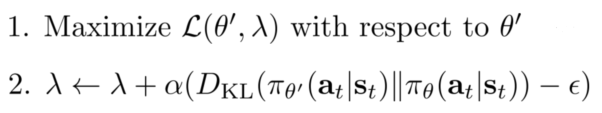
Where the first step can be imcomplete, i.e. we just need to to run a few gradient updates and go to step 2.

3.2 Natural Policy Gradient

Natural policy gradient was introduced much earlier than TRPO, but it turns out to be a special case of TRPO.

To ease the notation, let’s denote the objective as

\[\bar{A}(\theta') := \sum_t\mathbb{E}_{s_t\sim p_{\theta}(s_t)}\left[ \mathbb{E}_{a_t \sim q} \frac{\pi_{\theta'}(a_t\mid s_t)}{q(a_t\mid s_t)}\gamma^t A^{\pi_{\theta}}(s_t, a_t)\right]\]

The idea of natural policy gradient is to use linear approximation to the objective \(\bar{A}(\theta')\) and quadratic approximation to the constraint. This will lead to a very simple optimization problem that can be solved analytically by hand.

Use first order Taylor expension on \(\bar{A}(\theta')\), we have

\[\begin{align*} &\bar{A}(\theta') \\ &\approx \bar{A}(\theta) + \nabla_{\theta'}\bar{A}(\theta)^T(\theta' - \theta)\\ &\propto \nabla_{\theta'}\bar{A}(\theta)^T(\theta' - \theta) \end{align*}\]

Where we drop the constant in terms of \(\theta'\)

As a side note, we have

\[\begin{align} &\nabla_{\theta'}\bar{A}(\theta) \\ &= \sum_t\mathbb{E}_{s_t\sim p_{\theta}(s_t)}\left[ \mathbb{E}_{a_t \sim q} \frac{\pi_{\theta}(a_t\mid s_t)}{\pi_{\theta}(a_t\mid s_t)}\gamma^t \nabla_{\theta}\log \pi_{\theta'}(a_t\mid s_t) A^{\pi_{\theta}}(s_t, a_t)\right] \\ &= \sum_t\mathbb{E}_{s_t\sim p_{\theta}(s_t)}\left[ \mathbb{E}_{a_t \sim q} \gamma^t \nabla_{\theta}\log \pi_{\theta}(a_t\mid s_t) A^{\pi_{\theta}}(s_t, a_t)\right] \\ \end{align}\]

Which is actually the actor-critic policy gradient.

Then we expend the constraint to the second order

\[\begin{align*} D_\text{KL}(\pi_{\theta} \lVert \pi_{\theta'}) \approx \frac12 (\theta' - \theta)^T\nabla^2 D_\text{KL}(\pi_{\theta} \lVert \pi_{\theta'})(\theta' - \theta) \end{align*}\]

Where the constant and first order term can be shown to be both zeros. We can approximate the constraint using sample:

\[\{(s_t, a_t, r_t)\}_{t=0}^{T}\] \[\begin{equation}\label{second} \frac12 (\theta' - \theta)^T \left[\frac1T \sum_{t=1}^{T} \frac{\partial^2}{\partial \theta_i \partial \theta_j} D_\text{KL}(\pi_{\theta}(\cdot\mid s_t) \lVert \pi_{\theta'}(\cdot\mid s_t))\right](\theta' - \theta) < \delta \end{equation}\]

Where the KL term can usually be calculated analytically.

Also, since

\[\begin{equation*} \nabla^2 D_\text{KL}(\pi_{\theta} \lVert \pi_{\theta'}) = \mathbb{E}_{s_t\sim p_{\theta}(s_t)}\left[ \nabla_{\theta}\pi_{\theta}(a_t\mid s_t) \nabla_{\theta}\log\pi_{\theta}(a_t\mid s_t)^T \right] \end{equation*}\]

where the right hand side is the Fisher information matrix of \(\pi_{\theta}(a_t\mid s_t)\).

With this, we can also approximate the constraint by

\[\begin{equation}\label{fisher} \frac12(\theta' - \theta)^T \left[\frac1T \sum_{t=1}^{T} \frac{\partial}{\partial \theta_i}\log \pi_{\theta}(a_t\mid s_t) \frac{\partial}{\partial \theta_j}\log \pi_{\theta}(a_t\mid s_t)^T\right](\theta' - \theta)< \epsilon \end{equation}\]

Which approximation should we use? Equation \(\ref{second}\) use the fact that KL divergence of policy can usually be calculated analytically and therefore the MC estimator is more stable, but it requires taking second order derivative, which is not very compatible with automatic differentiation packages. Equation \(\ref{fisher}\) doesn’t require taking second order derivative, but it requires we store all the policy gradients along trajectories, also since we need to use single sample estimate to approximate the value of \(\log \pi_{\theta}(a_t\mid s_t)\), this approximate has larger variance.

Nevertheless, Since the course uses the fisher information matrix, we will follow it and express the contraint as

\[\begin{align*} \frac12 (\theta' - \theta)^T\mathbf{F}(\theta' - \theta)< \epsilon \end{align*}\]

With the objective:

\[\max_{\theta'} \nabla_{\theta}\bar{A}(\theta)^T(\theta' - \theta)\]

We can easily solve the constraint optimization by hand and arrive:

\[\theta' = \theta + \alpha \mathbf{F}^{-1}\nabla_{\theta}\bar{A}(\theta)\]

Where

\[\alpha = \sqrt{\frac{2\epsilon}{\nabla_{\theta}\bar{A}(\theta)^T\mathbf{F}\nabla_{\theta}\bar{A}(\theta)}}\]

4 Proximal Policy Optimization (PPO)

PPO is proposed to deal with the issues of TRPO while maintain it’s advantages. The component that makes TRPO stable is the trust region (i.e. the constraint), but the constraint optimization problem it leads to is difficult to solve.

Essentially PPO differs from TRPO by the way it formulize the trust region in optimization. Let

\[r_t(\theta') = \frac{\pi_{\theta'}(a_t\mid s_t)}{q(a_t\mid s_t)}\]

To makes sure the new and old policy are close, in TRPO, we formulize it as a constraint on the KL divergence; in PPO, we directly incorporate it in the object:

\[\begin{equation}\label{ppo_obj} \mathcal{L}^{\text{CLIP}} = \sum_t \mathbb{E}_{s_t,a_t \sim p_{\theta}(s_t, a_t)}\left[ \gamma^t \text{min}\left(r_t(\theta')A^{\theta}(s_t, a_t), \text{CLIP}(r_t(\theta'), 1-\epsilon, 1+\epsilon)A^{\theta}(s_t, a_t) \right) \right] \end{equation}\]

The first term in the min is the original TRPO objective (without incorporating the constraint). The clipping removes the incentive for moving \(r_t(\theta')\) outside of the interval \([1 − \epsilon, 1 + \epsilon]\). (the paper shows empirically that setting \(\epsilon=0.2\) gives best results). Since we take the “minimum of the clipped and unclipped objective, the final objective is a lower bound on the unclipped objective.” “With this scheme, we only ignore the change in probability ratio when it would make the objective improve, and we include it when it makes the objective worse.” (quoted sentences are directly from the PPO paper by Schulman et al. 17’).

Demo: OpenAI PPO

Link to the article by OpenAI