Deep RL 7 Q-learning
In this section we extend the online Q-iteration algorithm in the previous lecture by identifying the potential issues and introducing solutions. The improved algorithm can be very general and contains famous special cases such as DQN.
A little bit terminology: Q-learning and Q-iteration mean the same thing, the crucial part is if there is a “fitted” in front of them, when there is, that means the Q-function is approximated using some parametric function (e.g. a neural network).
to see the issues of online Q-iteration, let’s write out the algorithm:
- run some policy for one step and collect \((s, a, r, s')\)
- gradient update: \(\phi \leftarrow \phi - \alpha \frac{\partial Q_{\phi}(s,a)}{\partial \phi}\left(Q_{\phi}(s,a) - \left(r + \max_{a'}Q_{\phi}(s', a')\right)\right)\). Go to step 1.
The first issue with this algorithm is that, the transitions that are close to each other are highly correlated, this will lead to the Q-function to locally overfit to windows of transitions and fail to see broader context in order to accurately fit the whole function.
The second issue is that the target of the Q-function is changing very gradient step while the gradient doesn’t account for that change. To explain, for same transition \((s, a, r, s')\), when the current Q-function is \(Q_{\phi_1}\), the target is \(r + \max_{a'}Q_{\phi_1}(s', a')\), however, after one step of gradient update and the Q-function is \(Q_{\phi_2}\), the target also change to \(r + \max_{a'}Q_{\phi_2}(s', a')\). This is just like the Q-function is chasing it’s tail.
1 Replay Buffers
We solve issue one in this section. Note that as pointed out in the previous lecture, different from policy gradient methods which view data as trajectories, value function methods (including Q-iteration) view data as transitions which are snippets of trajectories. This means that the completeness of data as whole trajectories doesn’t matter in terms of learning a good Q-function.
Follow this idea, we introduce replay buffers, a concept that has been introduced to RL in the nineties.
A replay buffer \(\mathcal{B}\) stores many transition tuples \((s,a,s',r)\) which are collected ever time we run a policy during training (so the transitions doesn’t have to come from the same/latest policy). In Q-iteration, if the transitions are random samples from \(\mathcal{B}\) then we don’t have to worry about them being correlated. This gives algorithm:
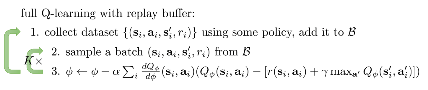
Note that the data in the replay buffer are still coming from the policies induced from the Q-iteration policy (original policy, epsilon greedy, or Boltzmann exploration etc.). It very common to just set \(K=1\), which makes the algorithm even more similar to the original online Q-iteration algorithm.
We can represent the algorithm using the following graph to make it more intuitive
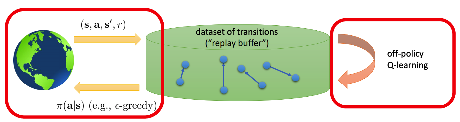
Since we are constantly adding new and possibly more relevent transitions to the buffer, we evict old transitions to keep the total amount of transtions in the buffer fixed.
In the rest of this lecture, we will always use replay buffers in any algorithms that we introduce.
2 Target networks
We deal with the second issue in this section. Instead of calculating the target always using the latest Q-function (which results in the Q-function chasing it’s own tail), we use a target network (also output Q-value) which is not too far from the latest Q-function, but fixed for a considerable amount of gradient steps.
Let’s see the Q-learning algorithm with both replay buffer and target network:
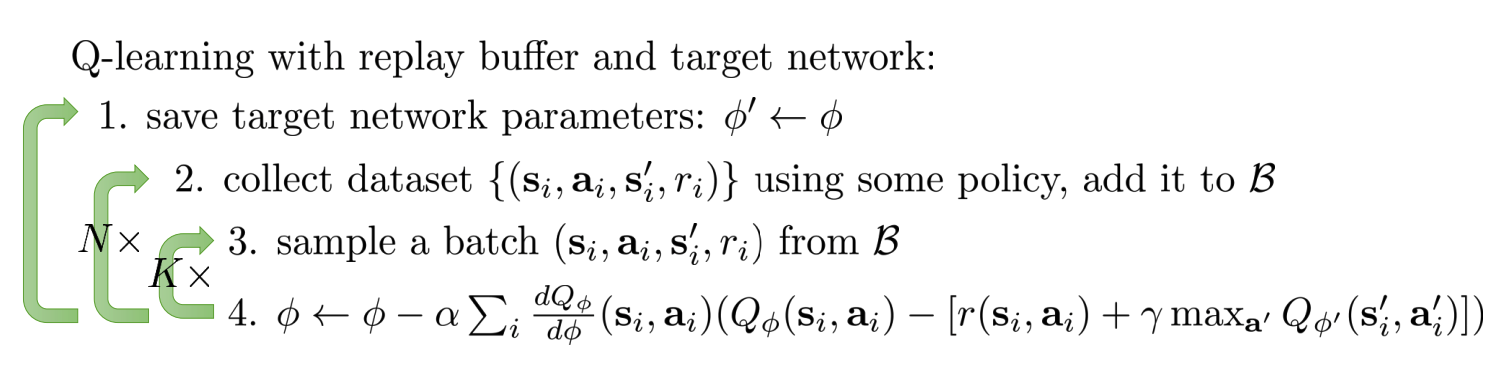
Note that the loop contains step 2, 3 and 4 is just plain regression, as the target network \(Q_{\phi'}\) is fixed within the loop. In practice, we usually set \(K\) to be between \(1\) and \(4\), while set \(N\) to be something like \(10000\).
As a specially case of the above algorithm, setting \(K = 1\) give us the famous classic DQN algorithm (Minh et al. 13’). We can switch step 1 and 2, and the resulting algorithm also works.
You might feel a little uncomfortable with this algorithm because after we just assign the target network parameters \(\phi'\) to be the current Q-function parameters \(\phi\), during the first few gradient steps, the lag between \(Q_{\phi'}\) and \(Q_{\phi}\) will be small, and as we update the Q-function \(Q_{\phi}\) in step 4, the lag become larger. We might not want the lag to be constantly changing during gradient update. To remedy this, we can use exponentially decaying moving average to update target network \(\phi'\) after every gradient update of \(\phi\) (or make N much smaller than \(10000\))
\[\phi' \leftarrow \tau \phi' + (1-\tau)\phi\]Where \(\tau\) can be some value that is very close to \(1\), such as \(0.999\)
For simplicity, we will sometimes just use “update \(\phi'\)” or “target update” in the remaining lecture, rather than specifying exactly how \(\phi'\) is updated.
3 Overestimation in Q-learning
This section is based on van Hasselt 10’ and van Hasselt et al. 15’.
Recall that using definition, we can derive the relation between value function and Q-function in Q-learning:
\[\begin{equation} \label{value} V(s) = \max_{a}Q(s,a) \end{equation}\]Since we don’t know the true Q-function, we need to estimate it using Monte Carlo samples.
Let’s use an simple example to show how we end up using the wrong estimator and overestimate \(\max_{a}Q(s,a)\).
Suppose there are three different actions that we can take \(a_1, a_2, a_3\), this means we need to estimate \(Q(s, a_1)\), \(Q(s,a_2)\), and \(Q(s, a_3)\) using their Monte Carlo samples and then take the max. For each value, we use
\[\begin{equation}\label{maxexp} \max\{ \mathbb{E}Q(s,a_1), \mathbb{E}Q(s,a_2), \mathbb{E}Q(s,a_3) \} \end{equation}\]and we will use one sample estimate to estimate equation \(\ref{maxexp}\)
\[\begin{equation}\label{esti} \max \{ Q_{\phi}(s,a_1), Q_{\phi}(s,a_2), Q_{\phi}(s,a_3) \}\end{equation}\]However, this is not unbiased estimator of equation \(\ref{maxexp}\), but an unbiased estimate of
\[\begin{equation} \label{expmax} \mathbb{E} \{\max\{ Q(s,a_1), Q(s,a_2), Q(s,a_3) \}\} \end{equation}\]Since we have
\[\mathbb{E} \{\max\{ Q(s,a_1), Q(s,a_2), Q(s,a_3) \}\} \geq \max\{ \mathbb{E}Q(s,a_1), \mathbb{E}Q(s,a_2), \mathbb{E}Q(s,a_3) \}\]Our estimator equation \(\ref{esti}\) will over estimate the target in equation \(\ref{value}\).
To make it even more concrete, consider the case where for all three actions, the true Q-values are all zero, but our estimated Q-values are
\[Q_{\phi}(s, a_1) = -0.1, Q_{\phi}(s, a_2) = 0, Q_{\phi}(s, a_3) = 0.1\]Then \(\max \{ Q_{\phi}(s,a_1), Q_{\phi}(s,a_2), Q_{\phi}(s,a_3) \} = 0.1\).
To see why \(\ref{esti}\) overestimates from another angle, the function approximation \(Q_{\phi}\) we are using is a biased estimate of \(Q\), and in equation \(\ref{esti}\), we use this \(Q_{\phi}\) to both estimate the Q-values and select the best Q-value, i.e.
\[\begin{equation} \max \{ Q_{\phi}(s,a_1), Q_{\phi}(s,a_2), Q_{\phi}(s,a_3) \} = Q_{\phi}(s,\text{argmax}_{a_i}\, \{ Q_{\phi}(s,a_1), Q_{\phi}(s,a_2), Q_{\phi}(s,a_3) \}) \end{equation}\]Thus the noise in \(Q_{\phi}\) will get accumulated and lead to overestimation.
This leads to one solution to the problem — Double Q-learning, which uses two different Q-functions for estimation and selection separately:
\[\begin{align} &a^* = \text{argmax}_{a}Q_{\phi_{select}}(s,a) \\ &\max_{a}Q(s,a) \approx Q_{\phi_{eval}}(s, a^*) \end{align}\]And if \(Q_{\phi_{select}}\) and \(Q_{\phi_{evak}}\) are noisy in different ways, the overestimation problem will go away!
So, we need to learn two neural networks? Well, that’s one possible way, but we can actually just use the current network as \(Q_{\phi_{select}}\) and the target network as \(Q_{\phi_{eval}}\). I.e.
\[\begin{align} &a^* = \text{argmax}_{a}Q_{\phi}(s,a) \\ &\max_{a}Q(s,a) \approx Q_{\phi'}(s, a^*) \end{align}\]These two networks are actually correlated, but they are sufficiently far away from each other (note that we assign the current network to the target network every 10000 or more gradient steps) that in practice this method works really well.
4 Q-learning with N-step Returns
This section is based on Munos et al. 16’.
In actor-critic lecture, we talked about the bias-variance tradeoff between estimating the expected sum of rewards using \(\sum_t \gamma^{t}r_t\) and \(r_t + \gamma V_{\phi}(s_{t+1})\). The former is a unbiased one sample estimate of the sum of return, which has high bias; the later is one step reward plus future rewards estimated by a fitted value value function, which can be biased but has less variance. Based on this, we can tradeoff bias and variance by using
\[\sum_{t'=t}^{t+N-1}\gamma^{t'-t}r_{t'} + \gamma^{N} V_{\phi}(s_{t+N})\]Where bigger \(N\) leads to smaller bias and higher variance.
Similarly, for Q-learning, we can estimate the target Q-value by
\[\begin{equation} \label{trade}y_t = \sum_{t'=t}^{t+N-1}\gamma^{t'-t}r_{t'} + \gamma^{N} \max_{a_{t+N}}Q_{\phi}(s_{t+N},a_{t+N})\end{equation}\]This seems ok at the first glance, but recall that \(y_t\) is estimating the Q-value under the current policy (our objective is to minimize \(\sum_t\left\|Q_{\phi}(s_t) - y_t\right\|^2\)), we need to make sure that the transitions \((s_{t'}, a_{t'},s_{t'+1})\) and rewards \(r_{t'}\) for \(t < t' \leq t+N-1\) come from running the current policy.
There are several ways to deal with this:
- Just ignore it and use whatever from the buffer. This actually often work well in practice.
- Compare every action along the trajectory with the action our current policy will take and set N to be the biggest number before the trajectory action and policy action disagree. This way, we change \(N\) adaptively to get only on-policy data. This works well when actual data are mostly on-policy, and action space is small.
- Importance sampling. Please see the original paper for detail.
5 Q-learning with Contiuous Actions
So far we’ve been assuming that \(\max_{a}Q_{\phi}(s,a)\) is tractable and fast operation, because it appears int the inner loop of Q-learning algorithms. This is true for discrete action space, where we can just parametrized the \(Q_{\phi}\) to take input \(s\) and output a vector of dimension \(\left\|\mathcal{A}\right\|\), where each entry of the vector is the Q-value for a specific action.
What if the action space is continuous?
We will briefly introduce three techniques that make Q-learning algorithms work in continuous actions space by making the operation \(\max_{a}Q_{\phi}(s,a)\) fast.
5.1 Randomized Search
The simplest solution is just randomly sample a bunch of actions and choose the one that gives the best estimated Q-value as the action we will take and the corresponding value as the value of the state, i.e.
\[max_{a}Q_{\phi}(s,a) \approx \max\{Q_{\phi}(s,a_1),Q_{\phi}(s,a_1),\cdots, Q_{\phi}(s,a_N)\}\]where \(a_i \sim \mathcal{A}\), \(\forall i=1:N\).
The advantages of this method is that it’s extremely simple and can be parallized easily, and the disadvantage is that it’s not very accurate, especially when the action space dimension is high.
There are other more complicated randomized search method such as cross-entropy method (we will introduce in detail in later lectures) and CMA-ES. However, these methods do not really work when the dimension of the action space is higher than \(40\).
5.2 Using Easily Maximazable Q-function Parameterization
We can easily find the maximal value of \(Q_{\phi}(s,a)\) is it is quadratic in \(a\). This leads to the Normalized Advantage Functions or NAFs (Gu et al. 16’), which parameterizes Q-function as
\[Q_{\phi}(s,a) = -\frac12 (a - \mu_{\phi}(s))^TP_{\phi}(s)(a - \mu_{\phi}(s)) + V_{\phi}(s)\]And the architecture is
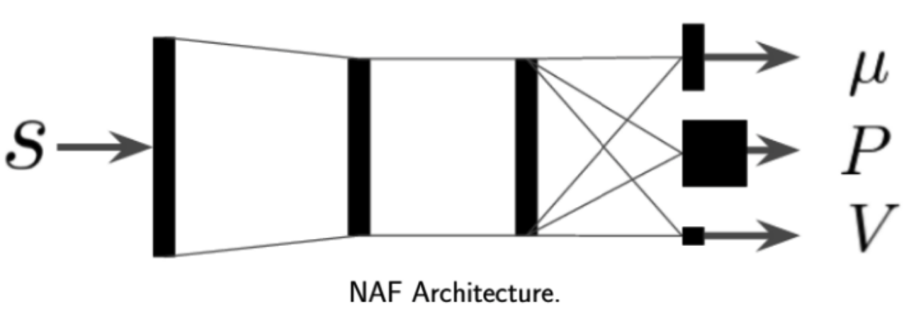
Where the network takes in state \(s\) and output vector \(\mu_{\phi}(s)\), positive-definite square matrix \(P_{\phi}(s)\) and scaler value \(V_{\phi}(s)\).
Using this parameterization, we have
\[\begin{align*} &\text{argmax}_a\,Q_{\phi}(s,a) = \mu_{\phi}(s)\\ &\max_a Q_{\phi}(s,a) = V_{\phi}(s) \end{align*}\]The disadvantage of this method is that the representation power is sacrificed because of the limited quadratic form.
5.3 Learn an Approximate Maximizer
Recall that in double Q-learning
\[max_{a}Q_{\phi'}(s,a) = Q_{\phi'}(s, \text{argmax}_a Q_{\phi}(s,a))\]the max operation can be fast if we can learn an approximate maximizer that output \(\text{argmax}_a Q_{\phi}(s,a)\). And this is the idea of Deep Deterministic Policy Gradient or DDPG (Lillicrap et al. 15’).
We parameterize the maximizer as a neural network \(\mu_{\theta}(s)\), that is to say we want to find \(\theta\) s.t.
\[\mu_{\theta}(s) = \text{argmax}_aQ_{\phi}(s,a)\]and therefore
\[max_{a}Q_{\phi'}(s,a) = Q_{\phi'}(s, \mu_{\theta}(s))\]This can be solved by stochastic gradient ascent with gradient update
\[\theta \leftarrow \theta + \beta \frac{\partial Q_{\phi}(s,a)}{\partial \mu_{\theta}(s)}\frac{\partial \mu_{\theta}(s)}{\partial \theta}\]To aviod the maximizer to chase its own tail similar to what happend to the Q-function in vanilla Q-learning, we use a target maximizer \(\theta'\) when assign
\[y = r + \gamma Q_{\phi'}(s', \mu_{\theta'}(s'))\]And update \(\theta'\) based on the current \(\theta\) by schedule during training.
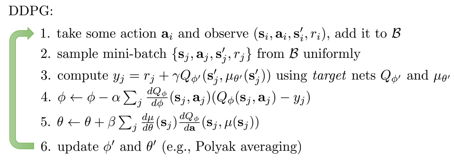
The algorithm of DDPG can be writen as
6 Tips for Praticioner
Here are some tips for applying Q-learnig methods
- Q-learning takes some care to stablize. Runs with different seeds might have inconsistent. Large replay buffer helps improve stability.
- It takes some time to start to work — might be no better than random for a while.
- Start with high exploration and gradually reduce.
- Bellman error gradients can be big; clip gradients or use Huber loss. (Bellman error is \(\left\|Q_{\phi}(s,a) - (r + \gamma\max_{a'}Q_{\phi'}(s',a')\right\|^2\))
- Double Q-learning helps a lot in practice, simple and no downsides.
- N-step returns also help a lot, but have some downsides (see previous section on N-step returns)/
- Schedule exploration (high to low) and learning rates (high to low), Adam optimizer can help too.