Deep RL 6 Value Function Methods

Previously we studied policy gradient methods, which proposes a parametric policy and optimize it to achieve better expected reward. Then we introduce actor-critic methods which augment the policy gradient with value functions and Q-function which reflects how good an action is at the current state compare to average (the advantage of an action). You might be thinking, if we have an advantage function that can tell us which action is good at every state, can we just act accroding to it?

You are right! A parametric policy is not needed if we have a good understanding of how good a state or action is. In this lecture, we will introduce methods that utilize the value functions or Q-functions to make decisions. In addition to CS285, part of this tutorial is based on CS287 Advanced Robotics by Professor Pieter Abbeel.

1 Value Iteration

Let’s assume the state space is discrete. Define

\(V^*_t(s)\): expected sum of rewards accumulated starting from state s, acting optimally for \(i\) steps

\(\pi^*_t(s)\): optimal action when in state s and getting to act for \(i\) steps

Note that we usually denote time index \(t\) as an subscript of state and action, but here for clarity we put them as subscript of \(V\) and \(\pi\).

The value iteration algorithm is the following:

1. Start with \(V_0^*(s) = 0\) for all state \(s\).
2. For \(t = 1,\cdots,T\):
   1. for all state \(s\):
      1. obtain state value \(\begin{equation}\label{value_update}V_{t+1}^*(s) \leftarrow \max_ar(s,a) + \gamma\mathbb{E}_{s'\sim p(s'\mid s, a)}V_t^*(s')\end{equation}\)
      2. obtain policy \(\pi^*_{t+1}(s) \leftarrow \text{argmax}_{a}\,r(s,a) + \gamma\mathbb{E}_{s'\sim p(s'\mid s, a)}V_t^*(s')\)

This algorithm is very stragtforward, at each time step and state, we just choose the action that give the highest Q-value and assign that value to be the value of the state. The policy is deterministic and because the way we obtain it, it is better than any policy for this state in terms of estimated Q-value. The update is called value update for Bellman update/back-up.

Value iteration is gauranteed to converge, and at convergence we have found the optimal value function \(V^*\) for the discounted infinite horizon problem, which satisfies the Bellman equations:

\[\forall s \in \mathcal{S}, V^*(s) = \max_a r(s,a) + \gamma\mathbb{E}_{s'\sim p(s'\mid s, a)}V^*(s')\]

which also tells us how to act, namely

\[\forall s \in \mathcal{S}, \pi^*(s) = \text{argmax}_a\, r(s,a) + \gamma\mathbb{E}_{s'\sim p(s'\mid s, a)}V^*(s')\]

Note that infinite horizon optimal policy is stationary, meaning that the optimal action at state \(s\) is the same for any time step (which means it’s efficient to store).

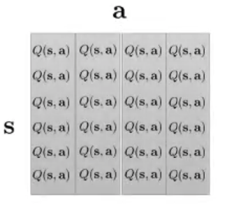
Note that Q-function is the only essential quantity, as value function is obtained by maximizing it w.r.t. action, and policy is obtained by argmaxing it w.r.t. action. As a very simple example, suppose that in our problem, both the state and action space are discrete and each contains 4 different choices like the following

At convergence, at each state, we can get the maximal value and the corresponding action like the following

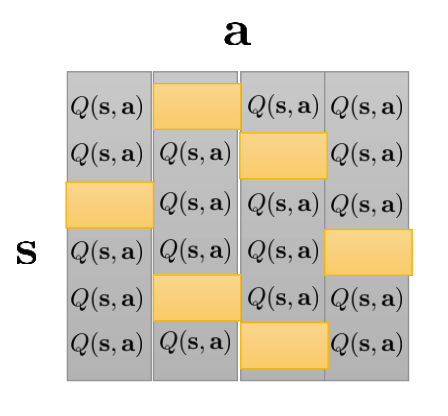
This table is the only thing we need in order to make decisions.

2 Policy Iteration

Policy iteration is an iterative algorithm that extends value iteration, it guarantees that the policy will improve at each iteration in terms of Q-value (Note that this is different from the previous likewise statement for value iteration which says the policy is better than any other policy for this state).

We first introduce policy evaluation. Suppose we now have a fix policy \(\pi(s)\) and want evaluate it. we can simply use the value update:

1. Start with \(V_0^*(s) = 0\) for all state \(s\).
2. For \(t = 1,\cdots,T\):
   1. for all state \(s\):
      1. obtain state value \(\begin{equation}\label{value_update_fix}V_{t+1}^*(s) \leftarrow r(s,\pi(s)) + \gamma\mathbb{E}_{s'\sim p(s'\mid s, a)}V_t^*(s')\end{equation}\)

And this is guaranteed to converge to the stationary infinite horizon value function, i.e. for state \(s\) the value is the same for any time step.

After value update, we do policy improvement:

1. for all state \(s\):
   1. \[\pi(s) \leftarrow \text{argmax}_{a}\, r(s,a) + \gamma\mathbb{E}_{s'\sim p(s'\mid s, a)}V_t^*(s')\]

Policy iteration is iteratively run policy evaluation and policy improvement. And like value iteration, policy iteration is also guaranteed to converge, and at convergence, the current policy and the value function is the optimal policy and value function.

Need to add better intuitive comparison between VI and PI, Need to add theoretical and empirical comparision between VI and PI.

3 Fitted Value Iteration and Q-iteration

One problem with vanilla value iteration and policy iteration is that the number of parameters is linear in the number of possible states, therefore, they are impractical for continuous state-space problem (or states are in a very fine-grained discrete space, i.e. RGB images).

If you went through the previous lecture, you will naturally think about using a neural net to fit the value function. This is called the fitted value iteration:

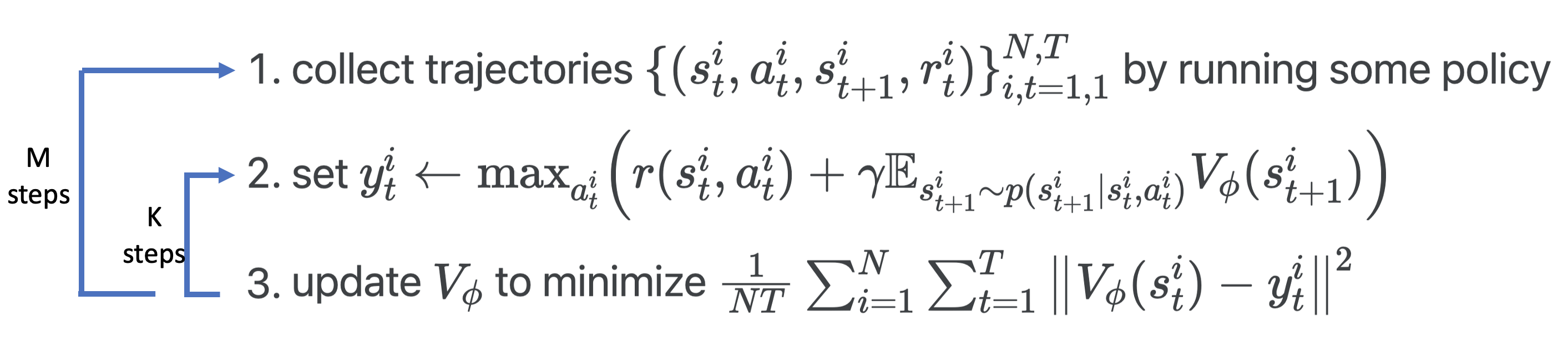
The problem with this algorithm is the second step. First, it’s very likely that the agent has been to any state at most once, which means we only have collected one action and corresponding reward for that state, and therefore given state \(s^i_t\), we cannot maximize over r(s^i_t, a^i_t) in terms of different actions i.e.

\[y^i_t \leftarrow \max_{a^i_t} \left(r(s^i_t, a^i_t) + \gamma\mathbb{E}_{s^i_{t+1}\sim p(s^i_{t+1}\mid s^i_t, a^i_t)}V(s^i_{t+1})\right)\]

shoule really be

\[y^i_t \leftarrow r^i_t + \max_{a^i_t}\gamma\mathbb{E}_{s^i_{t+1}\sim p(s^i_{t+1}\mid s^i_t, a^i_t)}V(s^i_{t+1})\]

Second, even if we move the max operation like above, since we don’t know the transition dynamics \(p(s^i_{t+1}\mid s^i_t, a^i_t)\), it’s pretty difficult to estimate the expectation term and therefore the maximization can be unreliable.

To get away from the above two issues, we instead fit the Q-function. First of all, there is no max operation involved in estimating the target Q-value

\[\begin{equation}\label{q1}Q(s,a) = r(s, a) + \gamma\mathbb{E}_{s'\dim p(s'\mid s, a)}V(s')\end{equation}\]

We still see \(V(s')\) here, but don’t worry, we always have \(V(s') = \max_{a'}Q(s', a')\) (or equivalently \(\pi(s') = \text{argmax}_{a'} \, Q(s', a')\) and recall that by definition \(V(s') =\mathbb{E}_{a'\dim\pi(a'\mid s')}Q(s',a')\)). Therefore, the equation \(\ref{q1}\) is equivalent to

\[\begin{equation}\label{q2}Q(s,a) = r(s, a) + \gamma\mathbb{E}_{s'\dim p(s'\mid s, a)}\max_{a'}Q(s', a')\end{equation}\]

Here we again don’t have transition dynamics so \(\mathbb{E}_{s'\dim p(s'\mid s, a)}\) needs to be estimated using samples. We can only use one sample estimation, i.e. the one in the sample trajectories that we have collected. This gives

\[\begin{equation}\label{q3}Q(s,a) \approx r(s, a) + \gamma\max_{a'}Q(s', a')\end{equation}\]

Note that in the equation above, \(s\), \(a\) and \(s'\) are the data that we collected, \(a'\) is a variable with respect to what we maximize the Q-function.

Using one sample estimation here is just like what we did in the previous lecture when fitting value function using bootstrap estimate. Q-function can be represented by neural network that takes in \(s\) and output a value for each possible action (e.g. there are \(10\) possible actions to take, then the output dimension is \(10\)), this makes it easier to do the max operation.

The above algorithm is called the fitted Q-iteration:

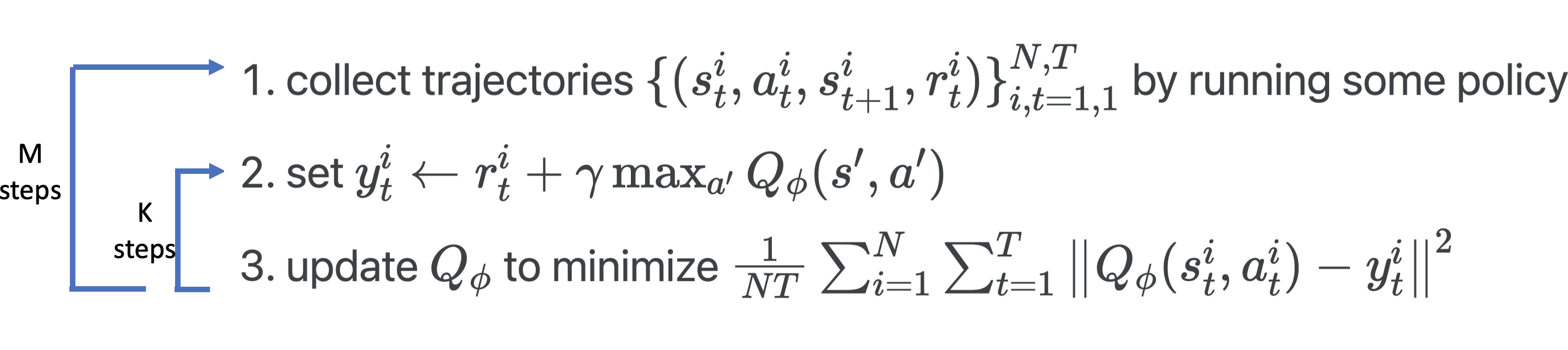
Or we can put it in the general RL algorithm framework:

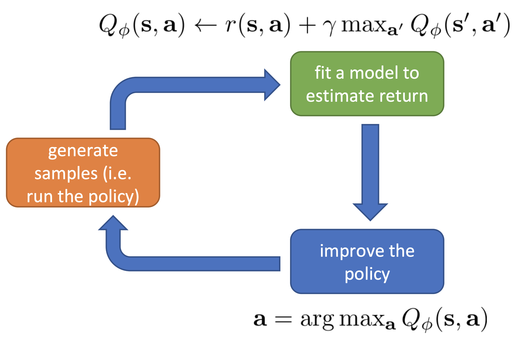
Note that the blue box is degenerated, meaning that we don’t explicitly go through this part in the algorithm.

Combine step 2 and 3 of the algorithm (or the just the green box), we see that fitted Q-iteration is actually looking for \(\phi\) that minimizes

\[\begin{equation}\mathcal{L} = \mathbb{E}_{(s,a,s') \sim p_{\text{data}}}\left\| Q_{\phi}(s,a) - (r(s,a) + \gamma \max_{a'}Q_{\phi}(s',a')\right\|^2\end{equation}\]

Where the difference in the norm is also referred to as the temporal difference error.

When the algorithm converges to \(\mathcal{L}=0\), we have \(Q_{\phi}(s,a) = (r(s,a) + \gamma \max_{a'}Q_{\phi}(s',a')\), \(\forall (s,a,s') \sim p_{\text{data}}\), we denote the Q-function as \(Q^*\), we have also found the optimal policy \(\pi^*\), where \(\pi^*(s) =\max_{a}Q_{\phi}(s,a)\).

However, the convergence of the algorithm is only guaranteed in the tabular case. You may wonder, it seems that step 3 can be done using gradient descentm, and then it’s just a regression problem, which should have many guarantees. But it’s actually not a vanilla gradient descent for regression, most of the time, the gradient of

\(\phi\) is taken to be \(\frac{1}{NT} \sum_{i=1}^{N}\sum_{t=1}^{T}\frac{\partial Q_{\phi}(s^i_t, a^i_t)}{\partial \phi}\left( Q_{\phi}(s^i_t, a^i_t) - y^i_t\right)\)

Note that \(y^i_t\) is a function of \(Q_{\phi}\), but we do not differentiate through it. You can actually manage to differentiate through it and get a read regression with gradient descent algorithm (which is call residual algorithm, see this link for more), but in general residual algorithm has some serious numerail issues and doesn’t work as well as vanilla Q-iteration.

Last thing to point out before we leave this section is that the Q-iteration algorithm is off-policy, the policy induced from Q-iteration is evolving all the time (policy is updated when we do \(\max_{a}Q_{\phi}(s,a)\)). Fitting Q-function requires only valid transition tuples \((s,a,s')\), which does not need to be generated by the newest policy. Essentially, for policy gradient and actor-critic algorithms, we view data as trajectories, while for value based methods, we view data as transition tuples, which are more flexible and contains less tightly bonded with any certain policy.

4 Online Q-iteration and Exploration

Similar to actor-critic algorithms, we also have an online version of the batch Q-iteration.

1. run some policy for one step and collect \((s, a, r, s')\)
2. set \(y \leftarrow r + \max_{a'}Q_{\phi}(s', a')\)
3. gradient update: \(\phi \leftarrow \phi - \alpha \frac{\partial Q_{\phi}(s,a)}{\partial \phi}(Q_{\phi}(s,a) - y)\). Go to step 1.

Here we ask the question, what policy should we use to collect data? Previous I mentioned that we do not have to use the latest deterministic policy derived from Q-function, and any valid transitions tuple will suffice. Well, actually, we want the training data to cover as much of the state-action space as possible. This is intuitive because we want the Q-function to cover more situations.

This is a bit on the opposite of the policy we obtained from Q-iteration. If we always generate data using latest Q-iteration policy, we might get stuck in some small subset of state-action space, because the agent will likely to always take the same action. To enable exploration, we modify the Q-iteration policy to make it probabilistic.

Here we introduce two simple (but effective) ways to do that, more sophistically methods will be introduced in later lectures.

Epsilon greedy

\[\begin{equation} \pi(a\mid s)= \begin{cases} 1-\epsilon,& \text{if } a = \text{argmax}_{a}\,Q(s,a)\\ \epsilon/(\|\mathcal{A}\|-1), & \text{otherwise} \end{cases} \end{equation}\]

Where \(\epsilon\) is a small number between \(0\) and \(1\), and \(\|\mathcal{A}\|\) is the number of actions in the action space. This stochastic policy allows the possibility to act differently than the best action according to the current Q-iteration policy. One possible disadvantage of this epsilon greedy policy is that the probabilities of taking actions other than the best action are all the same. Imagine at some point we already have a ok-ish Q-function, and for state \(s\), there are several actions that lead to high Q-value, if we are using epsilon greedy, then all good and bad actions have equal probability except for the one that give the biggest Q-value. This issue leads to the next policy.

Boltzmann Exploration

\[\begin{equation} \pi(a\mid s) \propto \exp{(Q_{\phi}(s,a))} \end{equation}\]

Under this policy, actions that of similar values will be even closer, i.e. similar probabilities of being selected.