
Deep RL 5 Actor Critic
Actor-critic algorithms build on the policy gradient framwork that we discussed in the previous lecture, but also augment it with learning value functions and Q-functions. The goal of this augmentation is still reducing variance, but from a slightly different angle.
Let’s take a look at the original policy gradient and it’s Monte Carlo approximator:
\[\begin{align} \nabla_{\theta}J(\theta) &= \mathbb{E}_{\tau\sim p_{\theta}(\tau)}\nabla_{\theta}\log \pi_{\theta}(a_t\mid s_t)r(s_t, a_t) \label{orig} \\ &\approx \frac1N \sum_{i=1}^{N}\left(\sum_{t=1}^{T}\nabla_{\theta}\log \pi_{\theta}(a^i_t\mid s^i_t)\right) \left(\sum_{t=1}^T r^i_t\right) \label{approx} \\ \end{align}\]In equation \(\ref{approx}\), \(N\) sample trajectories is used to approximate the expectation \(\mathbb{E}_{\tau\sim p_{\theta}(\tau)}\), but in equation \(\ref{approx}\) there are still one quantity that are approximated, i.e. the reward function \(r(r^i_t, a^i_t)\), and unfortuately, we are only using one sample \(r^i_t\) to approximate it.
Even with the use of causality and baseline, which gives
\[\begin{align}\label{var_red} \nabla_{\theta}J{\theta}&\approx\frac1N \sum_{i=1}^{N}\sum_{t=1}^{T}\nabla_{\theta}\log \pi_{\theta}(a^i_t\mid s^i_t) \left(\sum_{t'=t}^T r^i_t - b\right) \end{align}\]with \(b = \frac1N \sum_{i=1}^N\sum_{t'=t}^{T}r^i_t\), we are improving the variance in terms of expectation over trajectories (\(\mathbb{E}_{\tau\sim p_{\theta}(\tau)}\)) but not the estimation of reward to go (or better-than-average reward to go).
Actor-critic algorithms aims at better estimating the reward to go.
1 Fit the Value Function
We start by recalling the goal of reinforcement learning:
\[\begin{equation}\label{goal2}\text{argmax} \mathbb{E}_{p(\tau)}\sum_{t=1}^T r(s_t, a_t)\end{equation}\]Now define the Q-function:
\[\begin{align} Q^{\pi}(s_t,a_t) &= \mathbb{E}_{p_{\theta}}\left[\sum_{t'=t}^{T}r(s_{t'},a_{t'}) \mid s_t, a_t \right] \\ &= r(s_t, a_t) + \mathbb{E}_{a_{t+1} \sim \pi_{\theta}(a_{t+1}\mid s_{t+1}),s_{t+1}\sim p(s_{t+1}\mid s_t, a_t)} \left[ Q^{\pi}(s_{t+1}, a_{t+1}) \right] \end{align}\]Q-function is exactly the expected reward to go from step \(t\) given the state and action \((s_t, a_t)\).
How about the baseline \(b\) in \(\ref{var_red}\)? We can also replace it with lower variance estimate. To do that, we define the value function:
\[\begin{align} V^{\pi}(s_t) & = \mathbb{E}_{p_{\theta}}\left[\sum_{t'=t}^{T}r(s_{t'},a_{t'}) \mid s_t \right] \\ &= \mathbb{E}_{a_t\sim \pi_{\theta}(a_t\mid s_t)} \left\{ r(s_t, a_t) + \mathbb{E}_{s_{t+1} \sim p(s_{t+1}\mid s_t, a_t)}\left[ V^{\pi}(s_{t+1}) \right] \right\} \end{align}\]Value function measures how good the state is (i.e. the value of the state). This is exactly the expected reward of state averaged over different actions.
In addition, we define the advantage
\[\begin{equation} A^{\pi}(s_t, a_t) = Q^{\pi}(s_t, a_t) - V^{\pi}(s_t) \end{equation}\]In fact, \(\sum_{t'=t}^T r^i_t - \frac1N \sum_{i=1}^N\sum_{t'=t}^{T}r^i_t\) in equation \(\ref{var_red}\) looks very much just like the one sample estimate of the advantage \(A^{\pi}(s_t, a_t)\). In fact, \(\sum_{t'=t}^T r^i_t\) is an one sample estimate of The Q-function \(Q^{\pi}(s_t, a_t)\), however, \(\frac1N \sum_{i=1}^N\sum_{t'=t}^{T}r^i_t\) is not a estimate of \(V^{\pi}(s_t)\) (actually if the state space is continuous, we will only have an one sample estimate of \(V^{\pi}(s_t)\), which is also the \(\sum_{t'=t}^T r^i_t\), which is the same as the one sample estimate of \(Q^{\pi}(s_t, a_t)\). We only have an one sample estimate because we will never visit the state again). But \(V^{\pi}(s_t)\) is intuitively better than \(\frac1N \sum_{i=1}^N\sum_{t'=t}^{T}r^i_t\) even if we don’t consider the variance, because the former is the expected reward for state \(s_t\), and the later is an estimate of expected reward at time step \(t\) averaged over all possibly state. Since we want to know how good the action is in the current state, rather than in the current time step, we prefer the former.
If we have Q-function and value function, we can plug them in the original policy gradient and get the most ideal estimator:
\[\nabla_{\theta}J(\theta) = \frac1N\sum_{i=1}^N\sum_{t=1}^T \nabla_{\theta}\pi_{\theta}(a^i_t\mid s^i_t)\left(Q^{\pi}(s^i_t, a^i_t) - V^{\pi}(s^i_t)\right)\]However, we do not have \(Q^{\pi}(s_t, a_t)\) or \(V^{\pi}(s_t)\) and therefore we want to estimate them. Instead of using Monte Carlo estimate, we use function approximation, which might lead to a biased estimatio, but will give enormous variance reduction, in practice, the later usually brings more benefits than the hurts the former brings.
So we want to fit two neural networks to approximate \(Q^{\pi}(s_t, a_t)\) or \(V^{\pi}(s_t) separately\)? Well, it’s actually not necessary if we notice the relationship between the two functions:
\[\begin{equation}\label{relation} Q^{\pi}(s_t, a_t) = r(s_t, a_t) + \mathbb{E}_{s_{t+1} \sim p(s_{t+1}\mid s_t, a_t)}V^{\pi}(s_{t+1})\end{equation}\]And in practice we use one sample estimation to approximate \(\mathbb{E}_{s_{t+1} \sim p(s_{t+1}\mid s_t, a_t)}\), then we have
\[\begin{equation} Q^{\pi}(s^i_t, a^i_t) \approx r^i_t + V^{\pi}(s^i_{t+1})\end{equation}\]Therefore, we only need to fit \(V^{\pi}\). For training data, since \(V^{\pi}(s_t)=\mathbb{E}_{p_{\theta}}\left[\sum_{t'=t}^{T}r(s_{t'},a_{t'}) \mid s_t \right]\), ideally for every state \(s_t\), we want to have a bunch of differernt rollouts and rewards collected starting from that state, and then use the sample mean of rewards as the estimate of \(V^{\pi}(s_t)\). But this require reseting the simulator and actually impossible in the real world. Therefore, we have one sample estimator \(\sum_{t'=t}^Tr_{t'}\),
So, we use training data \(\{ (s^i_t, \sum_{t'}^Tr^i_{t'}) \}_{i=1,t=1}^{N, T}\) to train a neural network \(V^{\pi}_{\phi}\) in a supervised way. But we can further reduce the variance even if we only have one sample estimation of the expected reward — we can again apply the function approximation idea and replace \(\sum_{t'}^Tr^i_{t'}\) with \(r^i_t + V^{\pi}_{\phi'}(s^i_{t+1})\) in the training data, where \(V^{\pi}_{\phi'}\) is the previously fitted value function (i.e. \(\phi'\) is one gradient step before \(\phi\)). \(r^i_t + V^{\pi}_{\phi'}(s^i_{t+1})\) is called the Bootstrapp estimate of the value function. In summary, we fit \(V^{\pi}_{\phi}\) to \(V^{\pi}\) by minimizing
\[\begin{equation}\label{value_obj} \frac{1}{NT}\sum_{i,t=1,1}^{N,T}\left\|V^{\pi}_{\phi}(s^i_t) - y^i_t\right\|^2 \end{equation}\]where \(y^i_t = \sum_{t'}^Tr^i_{t'}\) or \(r^i_t + V^{\pi}_{\phi'}(s^i_{t+1})\) and the later usually works better.
With fitted value function \(V^{\pi}_{\phi}\), we can estimate the Q-function (Q-value) by
\[\hat{Q}^{\pi}(s^i_t, a^i_t) \approx r^i_t + V^{\pi}_{\phi}(s^i_{t+1})\]and therefore the advantage:
\[\hat{A}^{\pi}(s^i_t, a^i_t) = r^i_t + V^{\pi}_{\phi}(s^i_{t+1}) - V^{\pi}_{\phi}(s^i_t)\]And our actor-critic policy gradient is
\[\begin{align} \nabla_{\theta}J(\theta) &= \frac1N\sum_{i=1}^N\sum_{t=1}^T \nabla_{\theta}\pi_{\theta}(a^i_t\mid s^i_t)\left(Q^{\pi}(s^i_t, a^i_t) - V^{\pi}(s^i_t)\right) \\ &= \frac1N\sum_{i=1}^N\sum_{t=1}^T \nabla_{\theta}\pi_{\theta}(a^i_t\mid s^i_t)\left(r(s^i_t, a^i_t) + \mathbb{E}_{s_{t+1} \sim p(s_{t+1}\mid s^i_t, a^i_t)}V^{\pi}(s_{t+1}) - V^{\pi}(s^i_t)\right) \\ &\approx \frac1N\sum_{i=1}^N\sum_{t=1}^T \nabla_{\theta}\pi_{\theta}(a^i_t\mid s^i_t)\left(r^i_t + V^{\pi}_{\phi}(s^i_{t+1}) - V^{\pi}_{\phi}(s^i_t)\right) \\ &=\frac1N\sum_{i=1}^N\sum_{t=1}^T \nabla_{\theta}\pi_{\theta}(a^i_t\mid s^i_t)\hat{A}^{\pi}(s^i_t, a^i_t) \end{align}\]The batch actor-critic algorithm is:
- run current policy \(\pi_{\theta}\) and get trajectories \(\{ \tau^i \}_{i=1}^{N}\) and rewards \(\{ r^i_t \}_{i,t=1,1}^{N,T}\)
- fit value function \(V^{\pi}_{\phi}\) by minimizing equation \(\ref{value_obj}\)
- calculate the advantage of each state action pair \(\hat{A}^{\pi}(s^i_t, a^i_t) = r^i_t + V^{\pi}_{\phi}(s^i_{t+1}) - V^{\pi}_{\phi}(s^i_t)\)
- calculate actor-critic policy gradient \(\nabla_{\theta}J(\theta) =\frac1N\sum_{i=1}^N\sum_{t=1}^T \nabla_{\theta}\pi_{\theta}(a^i_t\mid s^i_t)\hat{A}^{\pi}(s^i_t, a^i_t)\)
- gradient update: \(\theta \leftarrow \theta + \alpha\nabla_{\theta}J(\theta)\)
We call it batch in that for each policy update we collect a batch of trajectories. We can also update the policy (and value function) using only one step of data i.e. \((s_t, a_t, r_t, s_{s+1})\), which leads to the online actor-critic algorithm which we will introduce later.
2 Discount Factor
Our previous discussion on policy gradient and actor-critic algorithms are all within the finite horizon or episodic learning scenario, where there is an ending time step \(T\) for the task. What about the infinite horizon scenario i.e. \(T = \infty\)?
Well in that case the original algorithm can run into problems because at the second step, \(V^{\pi}_{\phi}\) can get infinitely large in many cases. Or in vanilla policy gradient method, the sum of reward can get infinitely large.
To remedy that, we introduce the discount factor \(\gamma \in (0,1)\) and define the discounted expected reward, value function, and Q-function to be
\[\begin{align} J(\theta) &= \mathbb{E}_{\tau\sim p_{\theta}(\tau)}\sum_t \gamma^t r(s_t, a_t)\\ V^{\pi}(s_t) &= \mathbb{E}_{\tau_t \sim p_{\theta}(\tau_t)}\left[ \sum_{t'=t} \gamma^{t'-t}r(s_t', a_t') \mid s_t \right]\\ Q^{\pi}(s_t, a_t) &= \mathbb{E}_{\tau_t \sim p_{\theta}(\tau_t)}\left[ \sum_{t'=t} \gamma^{t'-t}r(s_t', a_t') \mid s_t, a_t \right]\\ &= r(s_t, a_t) + \gamma\mathbb{E}_{s_{t+1} \sim p(s_{t+1}\mid s_t, a_t)}V^{\pi}(s_{t+1}) \end{align}\]Therefore, the policy gradient and actor-critic policy gradient are \(\begin{align} \nabla_{\theta}J_{\text{PG}}(\theta) &= \frac1N \sum_{i=1}^N\sum_{t=1}\nabla_{\theta}\log \pi_{\theta}(a^i_t\mid s^i_t)\left(\sum_{t'=t}\gamma^{t'-t}r^i_{t'} - b\right) \label{dis_pg}\\ \nabla_{\theta}J_{\text{AC}}(\theta) &= \frac1N \sum_{i=1}^N\sum_{t=1}\nabla_{\theta}\log \pi_{\theta}(a^i_t\mid s^i_t)\left(r^i_t + \gamma V^{\pi}_{\phi}(s^i_{t+1}) - v^{\pi}_{\phi}(s^i_t)\right) \label{dis_ac} \end{align}\)
where in \(J_{\text{PG}}(\theta)\), \(b\) is also a discounted baseline e.g. \(\frac1N\sum_{i=1}^N\sum_{t'=t}\gamma^{t'-t}r^i_{t'}\).
Usually we set \(\gamma\) to be something like \(0.99\). It can be proved that discount factor can prevent the expected reward from being infinity and reduce the variance. Therefore, actually in most cases, no matter it’s finite of infinite horizon, people use discounted policy gradient, i.e. equation \(\ref{dis_pg} \text{ and } \ref{dis_ac}\), rather than the original ones.
3 Online Actor-critic algorithms
So far we’ve been discussing the batch actor-critic algorithm, which for each gradient update, we need to run the policy to collect a batch of trajectories. In this section, we introduce online actor-critic algorithms, which allow faster neural network weights update, and with some techniques can work better than batch actor-critic algorithms in some cases.
The simplest version of online actor-critic algorithm is similar to online learning, where instead of calculating the gradient using a batch of trajectories and rewards, it only uses one transition tuple \((s, a, s', r)\). The algorithm is the following:
- run policy \(\pi_{\theta}\) for one time step and collect \((s, a, s', r)\)
- gradient update \(V^{\pi}_{\phi}\) using (s, r + V^{\pi}_{\phi}(s’))$$
- evaluate \(\hat{A}^{\pi}(s) = r + \gamma V^{\pi}_{\phi}(s') - V^{\pi}_{\phi}(s)\)
- calculate policy gradient \(\nabla_{\theta}J(\theta) = \nabla_{\theta}\log \pi_{\theta}(a\mid s)\hat{A}^{\pi}(s)\)
- gradient update: \(\theta \leftarrow \theta + \alpha \nabla_{\theta}J(\theta)\)
However, this algorithm does not really work in most cases, because one sample estimate has very high variance, coupled with policy gradient, the variance can be notoriously high. To deal with the high variance problem, we introduce the synchronized parallel actor-critic algorithm, which is basically several agent running basic online actor-critic algorithm but using and updating the shared policy and value network \(\pi_{\theta} \text{ and } V^{\pi}_{\phi}\). See the following figure:

This can be very easily realized by just changing the the random seeds of the code.
Another variants which has been proved to work very well when we have a very large pool of workers is called the asynchronized parallel actor-critic algorithm:
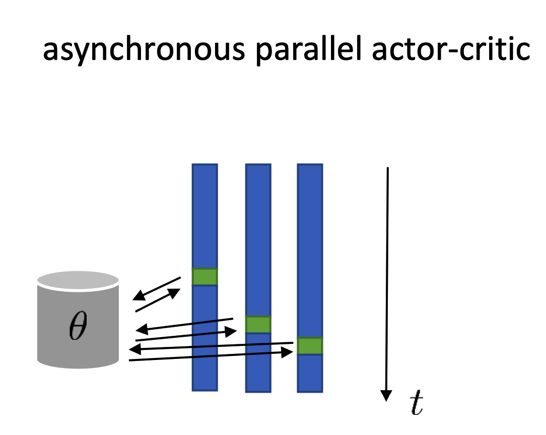
Each worker (agent) send the one step transition data to the center to update the parameters (both \(\theta\) and \(\phi\)), but do not wait for the updated weights to be deployed before it execute the next step in the environment. This is a little counterintuitive, because in this way, the worker might not using the latest policy to decide actions. But it turns out that the policy network will be very similar in the near time steps and since the algorithm is run asychronizely, it can be very efficient.
4 Variance/Bias Tradeoff in Estimating the Advantage
In this section we go back to the actor critic gradient, what distinguishes it from the vanilla policy gradient is that it uses the advantage \(\hat{A}^{\pi}(s_t, a_t)\) to replace the original one sample estimate of the expected discounted reward \(\sum_{t'=t}\gamma^{t'-t}r^i_{t'}\). The advantage has smaller variance, but it can be biased as \(V^{\pi}_{\phi}(s_{t})\) can be an imperfect estimation of the value function.
A question would be, can we bring the best from the two worlds and get a unbiased estimate of advantage while keep the variance low? Or further, can be develop a machanism that allows us to tradeoff the variance and bias in estimating the advantage?
The answer is yes and the rest of this section will introduce three advantage estimator that gives different variance bias tradeoff.
Recall that the original advantage estimator in actor-critic algorithm is:
\[\begin{align} \hat{A}^{\pi} &= \hat{Q}^{\pi}(s_t, a_t) - V^{\pi}_{\phi}(s_{t}) \\ &= r_t + \gamma V^{\pi}_{\phi}(s_{t+1}) - V^{\pi}_{\phi}(s_{t}) \label{orig_a} \end{align}\]4.1 critic as baseline (state dependent baseline )
The first advantage estimator is \(\begin{align} \hat{A}^{\pi} = \sum_{t'=t}^{T}\gamma^{t'-t}r_t - V^{\pi}_{\phi}(s_{t}) \end{align}\)
Compare to equation \(\ref{orig_a}\), we replace the neural estimation of discounted expected reward to go with the one sample estimaion \(\sum_{t'=t}^{T}\gamma^{t'-t}r_t\) used in policy gradient. This estimator has give lower variance than policy gradient whose baseline is a constant Greensmith et al. 04’ (but the variance is still higher than the actor-critic gradient). But is this advantage estimator really leads to an unbiased gradient estimator?
We can actually show that any state dependent baseline in policy gradient can lead to unbiased gradient estimator. I.e. we want to prove
\[\begin{align} \nabla_{\theta}J(\theta) &= \mathbb{E}_{\tau\sim p_{\theta}(\tau)}\sum_{t=1}^T\nabla_{\theta}\log \pi_{\theta}(a_t\mid s_t)\left( \sum_{t'=t}^{T}\gamma^{t'-t}r(s_{t'}, a_{t'}) - V^{\pi}(s_t)\right) \\ &= \mathbb{E}_{\tau\sim p_{\theta}(\tau)}\sum_{t=1}^T\nabla_{\theta}\log \pi_{\theta}(a_t\mid s_t)\sum_{t'=t}^{T}\gamma^{t'-t}r(s_{t'}, a_{t'}) \\ \end{align}\]let’s take one element from the summation \(\sum_{t=1}^T\) out:
\[\begin{align} \nabla_{\theta}J(\theta)_t &= \mathbb{E}_{\tau_t\sim p_{\theta}(\tau_t)}\nabla_{\theta}\log \pi_{\theta}(a_t\mid s_t)\left( \sum_{t'=t}^{T}\gamma^{t'-t}r(s_{t'}, a_{t'}) - V^{\pi}(s_t)\right) \\ &= \mathbb{E}_{\tau_t\sim p_{\theta}(\tau_t)}\nabla_{\theta}\log \pi_{\theta}(a_t\mid s_t)\left( \sum_{t'=t}^{T}\gamma^{t'-t}r(s_{t'}, a_{t'}) \right)- \mathbb{E}_{\tau_t\sim p_{\theta}(\tau_t)}\nabla_{\theta}\log \pi_{\theta}(a_t\mid s_t)V^{\pi}(s_t) \\ &= \mathbb{E}_{\tau_t\sim p_{\theta}(\tau_t)}\nabla_{\theta}\log \pi_{\theta}(a_t\mid s_t)\left( \sum_{t'=t}^{T}\gamma^{t'-t}r(s_{t'}, a_{t'}) \right) - \mathbb{E}_{s_{1:t}, a_{1:t-1}}V^{\pi}(s_t) \mathbb{E}_{a_t \sim \pi_{\theta}(a_t\mid s_t)}\nabla_{\theta}\log \pi_{\theta}(a_t\mid s_t) \\ &= \mathbb{E}_{\tau_t\sim p_{\theta}(\tau_t)}\nabla_{\theta}\log \pi_{\theta}(a_t\mid s_t)\left( \sum_{t'=t}^{T}\gamma^{t'-t}r(s_{t'}, a_{t'}) \right) - \mathbb{E}_{s_{1:t}, a_{1:t-1}}V^{\pi}(s_t) \cdot 0 \\ &= \mathbb{E}_{\tau_t\sim p_{\theta}(\tau_t)}\nabla_{\theta}\log \pi_{\theta}(a_t\mid s_t)\left( \sum_{t'=t}^{T}\gamma^{t'-t}r(s_{t'}, a_{t'}) \right) \end{align}\]4.2 state-action dependent baseline
To be updated, material is in Gu et al. 16’
4.3 Generalized Advantage Estimation (GAE)
Lastly let’s compare the advantage estimation introduced in section 4.1 (let’s call it \(A^{\pi}_{\text{MC}}\)) and the advantage estimation used in vanilla actor-critic algorithm (let’s call it \(A^{\pi}_{\text{C}}\))
\[\begin{align*} A^{\pi}_{\text{MC}} &= \sum_{t'=t}^{T}\gamma^{t'-t}r_t - V^{\pi}_{\phi}(s_{t}) \\ A^{\pi}_{\text{C}} &= r_t + \gamma V^{\pi}_{\phi}(s_{t+1}) - V^{\pi}_{\phi}(s_{t}) \end{align*}\]\(A^{\pi}_{\text{MC}}\) has higher variance because of the one sample estimation \(\sum_{t'=t}^{T}\gamma^{t'-t}r_t\), while \(A^{\pi}_{\text{C}}\) is biased because \(r_t + \gamma V^{\pi}_{\phi}(s_{t+1})\) might be an biased estimator of \(Q^{\pi}(s_{t+1})\).
Stare at these two estimators for a while, you might notice that the essential part that decide variance bias tradeoff is the estimation of \(Q^{\pi}\), one sample estimation has high variance while neural estimation can be biased. We can combine the two and use one sample estimation for the first \(n\) steps and use neural estimation for the rest. i.e.
\[\begin{align} A^{\pi}_{l} &= \sum_{t' = t}^{t+l-1} \gamma^{t'-t} r_{t'} + \gamma^{l} V^{\pi}_{\phi}(s_{t+l}) - V^{\pi}_{\phi}(s_{t}) \end{align}\]This also make sense intuitively, because the more distant from the current time step, the higher the variance will be. On the other hand, although \(V^{\pi}_{\phi}\) can be biased, when being multiplied by \(\gamma^{l}\), the effect can be small. Therefore, \(l\) controls the variance bias tradeoff of the advantage estimation. let \(l=1\), we recover \(A^{\pi}_{\text{C}}\), which has the highest bias and lowest variance, let \(l=\infty\), we recover \(A^{\pi}_{\text{MC}}\), which is unbiased by has the highest variance.
\(A^{\pi}_{GAE}\) is defined as a exponentially weighted sum of \(A^{\pi}_{l}\)’s:
\[\begin{equation}\label{form1} A^{\pi}_{GAE} = \sum_{l=1}^{\infty}w_l A^{\pi}_l \end{equation}\]where \(w_l \propto \lambda^{l-1}\)
It can be shown that \(A^{\pi}_{GAE}\) can be equivalently writen as
\[\begin{equation} A^{\pi}_{GAE} = \sum_{t'=t}^\infty (\gamma \lambda)^{t'-t} \delta_{t'} \end{equation}\]Where
\[\delta_{t'} = r_{t'} + \gamma V^{\pi}_{\phi}(s_{t'+1}) - V^{\pi}_{\phi}(s_{t'})\]