
Deep RL 2 Imitation Learning
The framework of imitation learning tackles reinforcement learning as a supervised learning problem.
1 Some Basic Notations and Terminologies
\(\begin{eqnarray*} &&o_t: \text{observation at time }t \\ &&a_t: \text{action at time }t \\ &&\pi(a_t\mid o_t): \text{policy, a distribution over actions }a_t\text{ given observation }o_t \\ &&p(o_t, a_t): \text{ marginal distribution of observation and action at time step } t \\ \end{eqnarray*}\)
More on policy \(\pi\)
When \(\pi(a_t\mid o_t)\) is a delta function, it’s a deterministic mapping from observation space to action space. In many cases we want to parameterize \(\pi\) by a neural net, and optimize the some objective to improve the policy. For example, when the action space is discrete, we can let \(\pi_{\theta}(a_t\mid o_t)= \text{Cat}(\alpha_{\theta}(o_t))\) and the neural net produces probabilities/logits of each category \((\alpha_{\theta}(o_t))\); when the action space is continuous, we can let \(\pi_{\theta}(a_t\mid o_t) = \mathcal{N}(\mu_{\theta}(o_t),\Sigma_{\theta}(o_t))\) and the neural network produces mean and variance of the Gaussian distribution.
2 Train a Policy by Supervised Learning
Suppose we want to train an agent to drive a car autonomously, in imitation learning framework, we first collect data \(\{(o_t,a_t)\}\) from human drivers, where ’s are the images from the car’s camera and ’s are the driver’s behaviors. We then parameterize policy \(\pi_{\theta}(a_t\mid o_t)\) by a neural network which takes in observation \(o_t\) and output action \(\hat{a}_t\). We want the neural net policy to act as close to human as possible, and therefore optimize the following objective:
\[\begin{equation}\label{eq:orig} \ell = \sum_{t}\mathcal{L}(\hat{a}_t, a_t) \end{equation}\]where \(\mathcal{L}\) can be mean square error (continuous action space), cross entropy (discrete action space) etc.
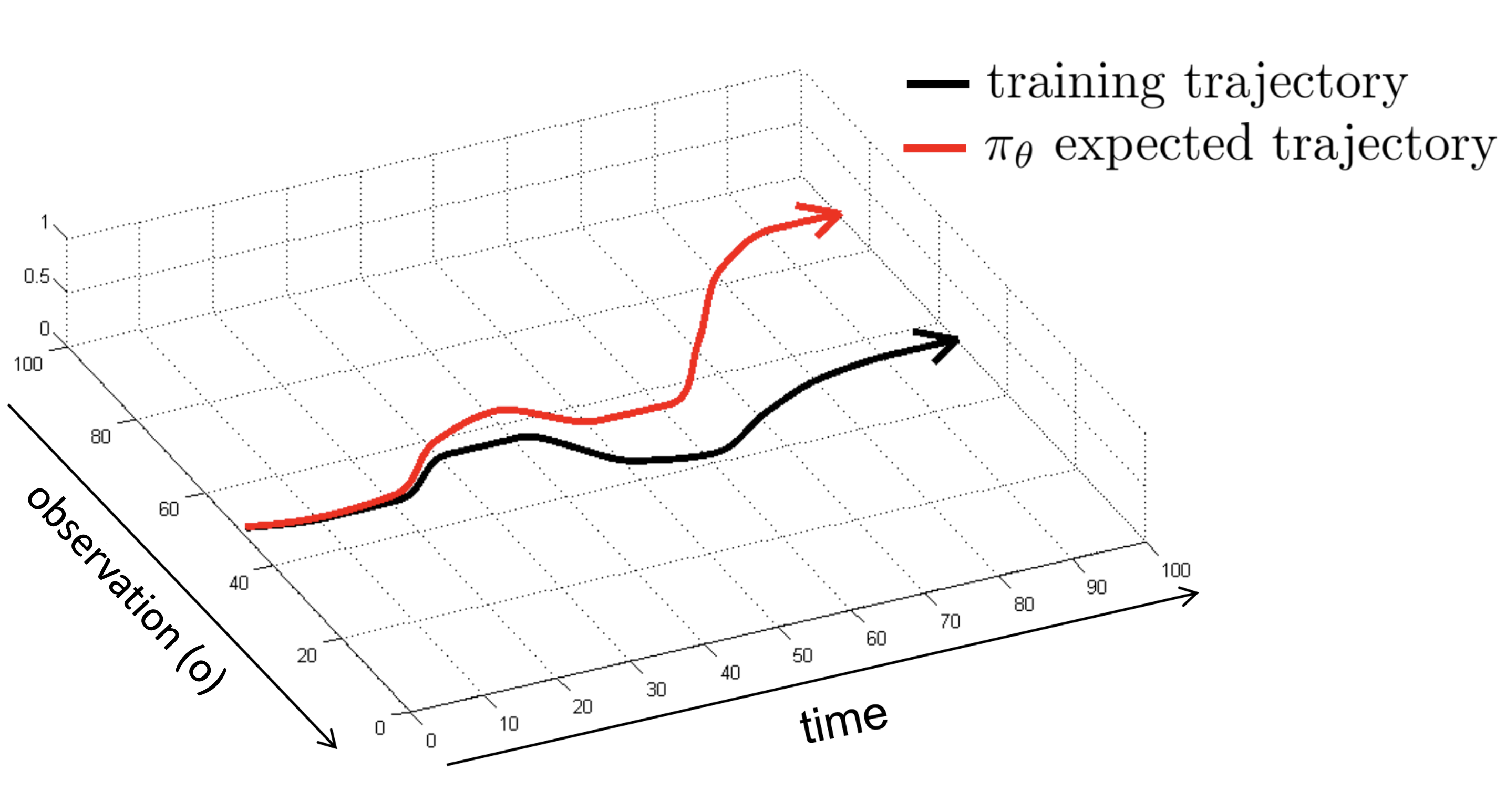
But this approach doesn’t really work and the reason is that when the agent takes actions based on \(\pi_{\theta}(a_t\mid o_t)\), as time goes on, the observations \({\pmb o} := (o_1, o_2, \cdots, o_t)\) can be very different than the trajectories in the training data and then it’s almost impossible for the learned policy \(\pi_{\theta}\) to be reliable because it has never seen the similar situations before. (Figures are all from CS285 (some are modified) unless otherwise pointed out)
One solution to this issue is to modify the data to introduce small mistakes and corrections, and therefore show the agent how to behave when it make small mistakes. For an example, see this NVIDIA paper.
3 Better data: DAgger
Here we focus on a more principled solution: DAgger or Dataset Aggregation (Ross et al. 11’). We introduce DAgger by first noticing that essential problem here is the distribution shift from \(p_{\text{data}}({\pmb o})\) and \(p_{\pi_{\theta}}({\pmb o})\). And the way Dagger deal with it is by collecting training data from \(p_{\pi_{\theta}}({\pmb o})\).
3.1 The algorithm
The algorithm of DAgger is the following:
-
Collect initial dataset \(\mathcal{D} = \{(o_t, a_t)\}_{t}\)
-
Supervised training for \(\pi_{\theta}(a_t\mid o_t)\) using \(\mathcal{D}\)
-
Run \(\pi_{\theta}(a_t\mid o_t)\) to get observations \(\{(o^{\pi}_t)\}_{t}\)
-
Ask human to label \(\{(o^{\pi}_t)\}_{t}\) to get \(\mathcal{D}^{\pi} = \{(o^{\pi}_t, a_t)\}_{t}\)
-
Aggregate dataset: \(\mathcal{D} \leftarrow \mathcal{D} \cup \mathcal{D}^{\pi}\), go to step 2.
For an example of using DAgger to fly drones, please see Ross. et al. ‘12.
3.2 Theoretical analysis of DAgger
Now let do some analysis of this algorithm! The analysis follows lecture 2 where they replaced observation \(o_t\) by state \(s_t\) everywhere, this is a bit strange, and my guess is that there are really used interchangeably in this lecture, in future lectures, observations are much less seen. Here we will stick to \(\pi_{\theta}(a_t\mid o_t)\)
Assume human decision or optimal policy is \(\pi^*(o_t)\) (which does not has to be deterministic, it can be a set that contains the decisions that human make given observation \(o_t\), here fore brevity we treat it as deterministic), and the cost \(c(o_t, a_t)\) is binary:
\[\begin{equation}\label{eq:cost_fn}c(o_t, a_t) = \begin{cases} 0,& \text{if } a_t = \pi^*(o_t)\\ 1, & \text{otherwise} \end{cases} \end{equation}\]Our goal is to find \(\theta^*\) such that it minimizes \(\begin{equation}\label{eq:goal} \mathbb{E}_{(o_t, a_t) \sim p_{\theta}(o_t, a_t)}\sum_t c(o_t, a_t) \end{equation}\)
By running DAgger, we assume \(\pi_{\theta}(a_t\mid o_t)\rightarrow \pi_{\text{train}}(a_t\mid o_t)\), therefore the joint distribution \(p_{\theta}(o_t, a_t) \rightarrow p_{\text{train}}(o_t, a_t)\). Mathematically, we assume
\[\begin{equation}\label{eq:assump} \forall s \in p_{\text{train}}(s), \pi_{\theta}(a\neq \pi^*(o_t)\mid s) \leq \epsilon\end{equation}\]Then we have
\[\begin{equation}\label{eq:p_dist} p_{\theta}(o_t, a_t) = (1-\epsilon)^{(t+1)}p_{\text{train}}(o_t, a_t) + \left( 1 - \left(1-\epsilon\right)^{(t+1)} \right)p_{\text{mistake}}(o_t, a_t)\end{equation}\]To understand the equation \(\ref{eq:p_dist}\), start from \(s_0\), suppose the agent keeps acting the same as humans at each time step (which has probability \(1-\epsilon\)), then at time step \(t\), the joint distribution \(p_{\theta}(o_t, a_t)\) will be the same as \(p_{\text{train}}(o_t, a_t)\) the probability for this event to happen is \((1-\epsilon)^{(t+1)}\), while if the agent did anything different then humans along the way, the joint distribution at time step \(t\) might be different, which we denote as \(p_{\text{mistake}}(o_t, a_t)\). Note that \(p_{\text{mistake}}(o_t, a_t)\) can also be the same as \(p_{\text{train}}(o_t, a_t)\), but it doesn’t affect our analysis.
From equation \(\ref{eq:p_dist}\), we can derive:
\[\begin{eqnarray}\label{eq:p_dist2} &&\left|p_{\theta}(o_t, a_t) - p_{\text{train}}(o_t, a_t)\right| \\ &=& \left( 1 - (1-\epsilon)^{(t+1)} \right)\left|p_{\text{mistake}}(o_t, a_t) - p_{\text{train}}(o_t, a_t)\right| \nonumber \\ &=& \left( 1 - (1-\epsilon)^{(t+1)} \right)\cdot 2 \quad \text{(suppose state are discrete)} \nonumber \\ &=& 2\epsilon (t+1) \quad \text{(}\forall \epsilon\in[0,1] (1-\epsilon)^{(t+1)} \geq 1-\epsilon (t+1)\text{)} \end{eqnarray}\]Now, lets bound the inference cost, i.e. our goal equation \(\ref{eq:goal}\)
\[\begin{eqnarray}\label{eq:cost_bound} &&\mathbb{E}_{(o_t, a_t) \sim p_{\theta}(o_t, a_t)}\sum_t c(o_t, a_t) \\ &=& \sum_t \mathbb{E}_{p_{\theta}(o_t, a_t)}c(o_t, a_t) \\ &=& \sum_t\sum_{o_t}p_{\theta}(o_t, a_t)c(o_t) \\ &\leq& \sum_t\sum_{o_t}p_{\text{train}}(o_t)c(o_t, a_t) + \left| p_{\theta}(o_t, a_t) - p_{\text{train}}(o_t) \right|c_{\text{max}} \\ &\leq& \sum_t \mathbb{E}_{p_{\text{train}}(o_t,a_t)}c(o_t, a_t) + \left| p_{\theta}(o_t, a_t) - p_{\text{train}}(o_t) \right|c_{\text{max}} \\ &\leq& \sum_t (0 + 2\epsilon (t+1)) \\ &\leq& \epsilon T(T+1) \\ &=&O(\epsilon T^2) \end{eqnarray}\]4 Better Policy: Non-markovian Policy and Multimodal Policy
To solve the distribution shift problem, i.e. \(p_{\theta}(o_t, a_t)\) versus \(p_{train}(o_t, a_t)\), DAgger makes state sequence in training trajectory close to the state sequence during inference time (the state sequence we will encounter when acting based on the learn policy). Instead, we can improve the policy itself that such \(\pi_{\theta}(a_t\mid o_t)\) is very close to \(\pi^*(a_t\mid o_t\). For inspiration of what to improve, we consider the potential issue of using a conventional neural net (e.g. a CNN) as \(\pi_{\theta}\).
4.1 make decisions based on only current observation
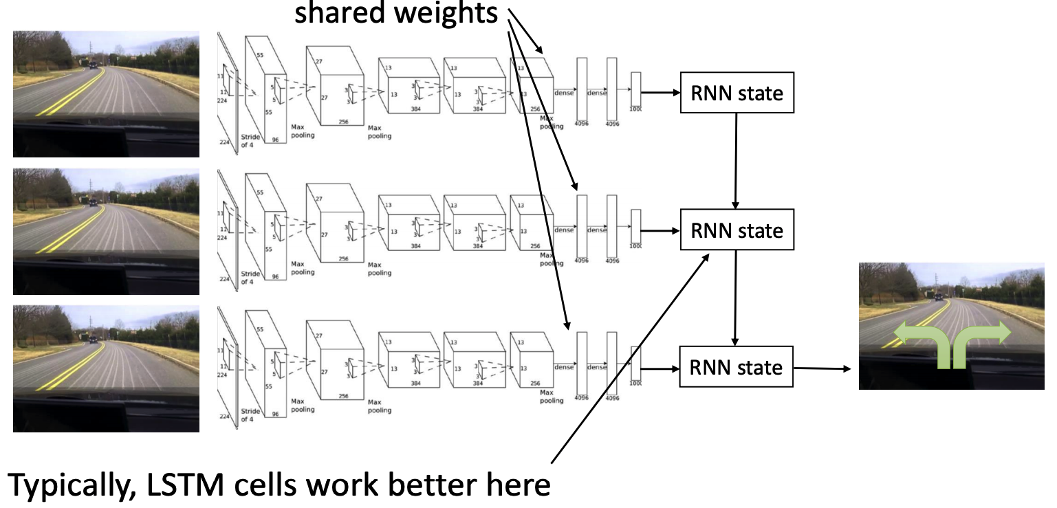
\(\pi_{\theta}(a_t\mid o_t)\) means we take action based on the current observation, but this is usually not how human make decisions. Therefore, for better decision making, we consider \(k\) past observations, i.e. let policy be \(\pi_{\theta}(a_t\mid o_t, \cdots, o_{t-k+1})\). One example in self-driving car is to use a CNN to process image (the \(o_t\)’s), and sequantially pass the image features to a RNN, and use the e.g. final state of the RNN to produce a desicion (\(a_t\)). A figure is shown below:
However, this might actually lead to an issue called causal confusion, which basically means the agent get confused about which observation lead the human to take that action and thus it can make wrong decision with high confidence. For more detailed illustrate about causal confusion, please see de Haan et al. 19’.
4.2 unimodal distribution for continuous action space
For humans, in any given situation, there are usually several possible actions to take and those actions don’t not have to be similar to each other. But when we parameterize policy as a unimodal Guassian distribution, it’s difficult for it to exhibit the multimodality behavior. To deal with that, there are three popular methods:
4.2.1 Mixture of Guassians
This is selfexplanatory, just parameterize the distribution as a mixture of Guassian distributions:
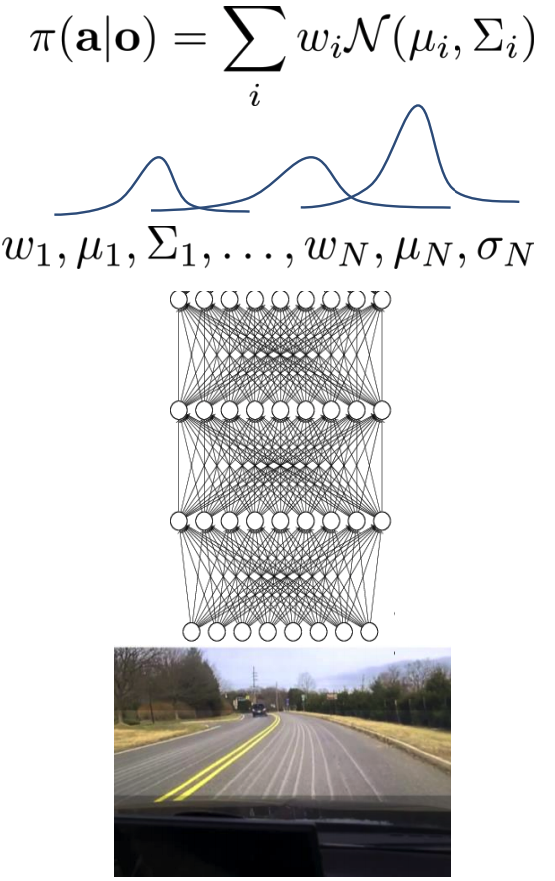
Where weights \(w_n\), means \(\mu_n\), and covariance matrices \(\Sigma_n\) are all output of the neural net.
4.2.2 Latent variable models
an example is to use a variational autoencoder type of model, which means to generate a output, in addition to using the input image (observation \(o_t\)), we also use a sample from a simple distribution (e.g. standard Guassian). Therefore, even if the input image is the same, different Gaussian samples can lead to different output distribution. Actually people have shown that such a model can represent any distributions. reference needed
4.2.3 Autoregressive discretization
If the action space is discrete, we just need to let the neural net to output the logits of different actions and multimodality is not a problem. However, if we were to simply discretize the action space and model them using neural net, there will be an exponential explosion in the number of parameters of the last layer. For example, if the action space is \(n\) dimensional, and for each dimension, we will discritize it into \(m\) bins, therefore, the number of logits needed to represent this discrete distribution is \(m^n\) which can be impractical when \(n\) gets beyound single digit.
To get away with this exponential explosion problem, we use factor the distribution \(\pi_{\theta}({\pmb a}\mid o) = p_{\theta_1}(a_1\mid o)\prod_{i=2}^{n}p_{\theta_2}(a_i\mid o, a_{i-1})\). Here we only need two different network parameterized by \(\theta_1\) and \(\theta_2\) (or even just one if we let \(a_0=0\) and let \(\pi_{\theta}({\pmb a}\mid o) = \prod_{i=1}^{n}p_{\theta_2}(a_i\mid o, a_{i-1})\)) and the number of parameters of the network is \(m\). Since we predict the next dimension of the action space in a autoregressive way, we name the method autoregressive discretization.
To be continued…
5 Few Shot Imitation Learning
Goal conditioned behavior cloning. example: learning latent plans from play