
Deep RL 3 Intro to RL
This is an introduction to reinforcement learning, including core concepts, the general goal, the general framework, introduction and comparison of different types of approaches. This section contains nighty percent of the materials that are going to be covered by this course.
1 Notations and Terminologies
We have introduced some of the notations in lecture 2. Here we give a more comprehansive introduction of the core concepts in reinforcement learning。
Reinforcement learning centers around the Markov Decision Processes (MDPs): \(\mathcal{M} = \{ \mathcal{S}, \mathcal{A}, \mathcal{T}, r \}\) with the four terms defined as:
\[\begin{eqnarray*} &&\mathcal{S} \text{ is state space, state } s \in \mathcal{S} \text{ can be discrete or continuous} \\ &&\mathcal{A} \text{ is action space, action } a \in \mathcal{A} \text{ can be discrete or continuous} \\ &&\mathcal{T} \text{ is the transition operator } \\ &&r: \mathcal{S}\times\mathcal{A} \to \mathbb{R} \text{ is the reward function, specify how good the state and action is} \end{eqnarray*}\]More on the transition operator \(\mathcal{T}\), denote
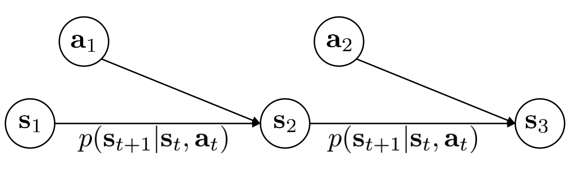
\[\begin{eqnarray*} &&\mu_{j} := p(s = j), t \text{ can be } \\ &&\xi_{k} := p(a = k) \\ &&\mathcal{T}_{i,j,k} := p(s' = i\mid s=j, a=k)\\ &&\text{we have } \mu_{i} = \sum_{j,k}\mathcal{T}_{i,j,k}\mu_{j}\xi_{k} \\ \end{eqnarray*}\]The transition operator explains why the process is call Markov Decision Processes, this is because the state sequence has first order markov property, i.e. suppose \(s'\) is the subsequent state of \(s\), than \(s'\) is independent of any previous state given \(s\). A grapical model of MDPs is
For simplicity, we illustrate the transition operator using discrete state and action space. I didn’t find any illustration for the continuous case. Actually trainsition operator is rarely used in this course, most of the time we just use the transition probability \(p(s'\mid s,a)\) (more often writen as \(p(s_{t+1}\mid s_t, a_t)\)). To avoid confusion, the community also refer to the transition probability as model, dynamics, or transition dynamics.
Another process that is also common in reinforcement learning is called Partially Observed Markov Decision Processes (POMDPs): \(\mathcal{M} = \{ \mathcal{S}, \mathcal{A}, \mathcal{O}, \mathcal{T}, \mathcal{E}, r \}\)
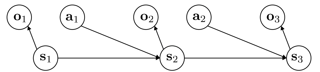
\[\begin{eqnarray*} &&\mathcal{S} \text{ is state space, state } s \in \mathcal{S} \text{ can be discrete or continuous} \\ &&\mathcal{A} \text{ is action space, action } a \in \mathcal{A} \text{ can be discrete or continuous} \\ &&\mathcal{O} \text{ is observation space, observation } o \in \mathcal{O} \text{ can be discrete or continuous} \\ &&\mathcal{E} \text{ the set for emission probability }p(o\mid s) \\ &&\mathcal{T} \text{ is the transition operator } \\ &&r: \mathcal{S}\times\mathcal{A} \to \mathbb{R} \text{ is the reward function, specify how good the state and action is} \end{eqnarray*}\]Comapre to MDPs, POMDPs have two more terms, observation space \(\mathcal{O}\) and emission probability set \(\mathcal{E}\). State sequence still satisfies first order Markov property, but it’s not observable. We can only observe observation \(o\) which doesn’t satisfy markov property. The model/dynamics is still on states and actions rather than on observations and actions, i.e. \(p(s'\mid s,a) \text{ rather than } p(o'\mid o,a)\) and we have one addition probability distribution to worry about which is the emission probability \(p(o\mid s)\). The graphical model for POMDPs is shown below:
In the previous section on imitation learning, we define policy as \(\pi_{\theta}(a_t\mid o_t)\). This is actually a more general case compare to \(\pi_{\theta}(a_t\mid s_t)\), as observation sequence doesn’t satisfy first order Markovian property.
In the course, they use an example to show the difference between \(o_t\) and \(s_t\):
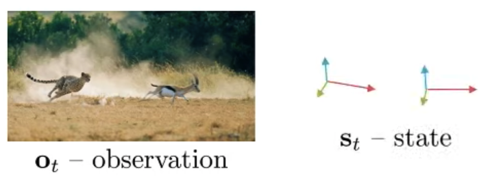
But throughout the course (also in coding homework), they actually treat observation directly as state :)
In this course, we will mainly consider MDPs. We even use the observations (i.e. sensory measurements like images) during learning as the state in MDPs.
2 The Goal of Reinforcement Learning
Before presenting the goal of reinforcement learning, we have one more very important concept to introduce — trajectory \(\tau:=(s_1, a_1, s_2, a_2, \cdots, s_T, a_T)\). In MDPs, we can write out the distribution of \(\tau\):
\[\begin{equation}\label{traj_dist}p_{\theta}(\tau) = p_{\theta}(s_1, a_1, \cdots, s_T, a_T)= p(s_1)\prod_{t=1}^{T}\pi_{\theta}(a_t\mid s_t)p(s_{t+1}\mid s_t, a_t)\end{equation}\]This distribution can also be writen as \(p_{\theta}(\tau) = \prod_{t=1}^{T}p_{\theta}(s_{t+1}, a_{t+1}\mid s_t, a_t)\), where \(p_{\theta}(s_{t+1},a_{t+1}\mid s_t, a_t) = p(s_{t+1}\mid s_t, a_t)\pi_{\theta}(a_{t+1}\mid s_{t+1})\)
The goal of reinforcement learning is to find the best policy to maximize the expected reward, i.e.
\[\begin{align} \theta^* &= \text{argmax}_{\theta} \mathbb{E}_{\tau\sim p_{\theta}(\tau)}\sum_{t=1}^T r(s_t, a_t) \label{eq:goal1}\\ &= \text{argmax}_{\theta} \sum_{t=1}^T \mathbb{E}_{(s_t,a_t) \sim p_{\theta}(s_t, a_t)}r(s_t, a_t) \label{eq:goal2} \end{align}\]What if \(T = \inf\)? In this case the above optimization is over an expectation of infinite summation or infinite summation of an expectation! However, if \(p_{\theta}(s_t, a_t)\) converge to an stationary distribution \(p_{\theta}(s,a)\), we can optimize the following as our goal:
\[\begin{equation}\label{eq:goal3} \theta^* = \text{argmax}_{\theta} \mathbb{E}_{(s,a) \sim p_{\theta}(s, a)}r(s, a)\end{equation}\]This is because when \(T = \inf\), \(r(s,a)\) where \(s\) and \(a\) are from the stationary distribution \(p_{\theta}(s,a)\) will dominate the summation in equation \(\ref{eq:goal2}\) (because there are infinite many of them!). And therefore, equation \(\ref{eq:goal3}\) is asymtotically equivalent to equation \(\ref{eq:goal2}\).
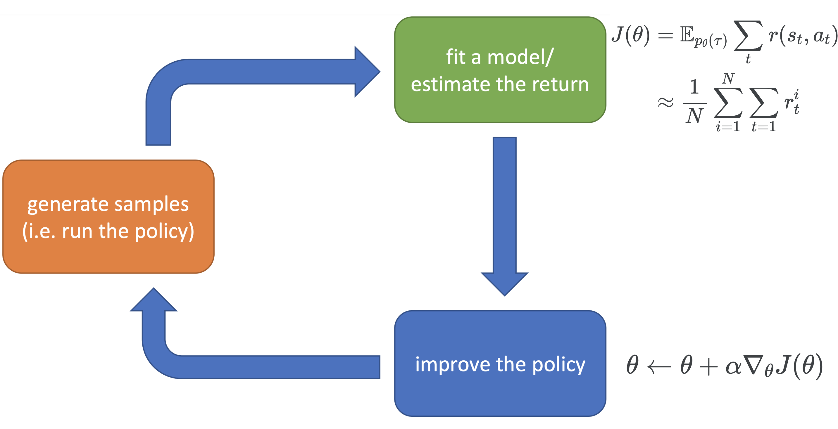
3 The Framework of RL Algorithm
Most of the RL algorithm can be framed as the following plot:
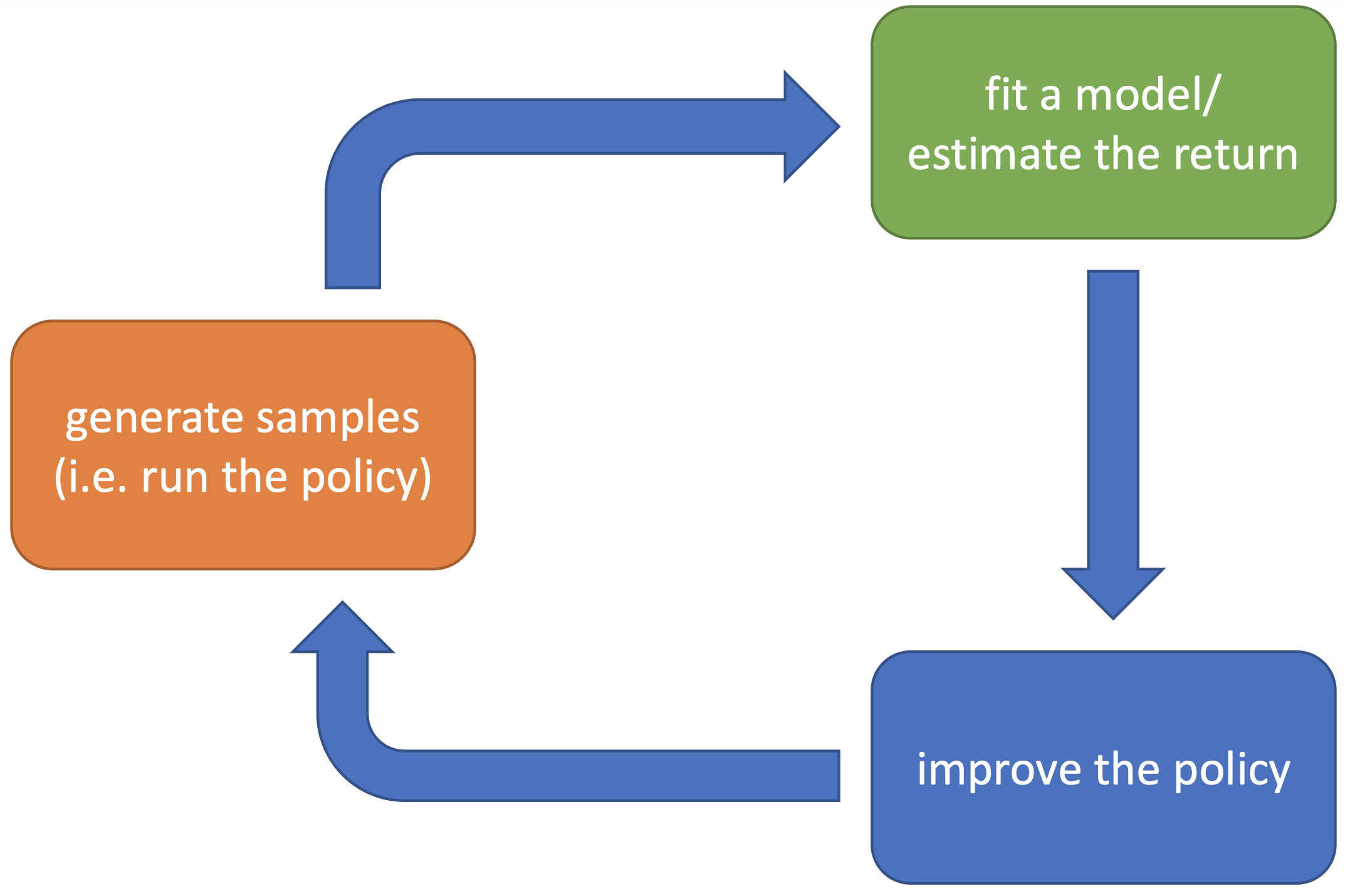
This is a loop, but let’s start with the orange box — generate samples, just as supervised learning and unsupervised learning, data is the fuel for reinforcement learning. The samples are trajectories i.e. \(\{\tau_i\}_{i=1}^{N}\) where \(\tau_i = (s^i_1, a^i_1, \cdots, s^i_T, a^i_T)\) is one trajectory, and rewards i.e. \(\{ r^i \}_{i=1}^{N}\), where \(r^i_t = (r^i_1, \cdots, r^i_T)\) (\(T\) doesn’t have to be the same for every trajectory). The trajectories are typically obtained from the trajectory distribution \(p_{\theta}(\tau)\) which is induced by policy \(\pi_{\theta}(a_t\mid o_t)\) (shown in equation \(\ref{traj_dist}\)), which means trajectores are obtained by runnig the policy. Note that there are other ways to get trajectories such as using exploration methods. Rewards are obtained from the environment (real environment or simulator), and the reward function is unknown to the agent. Although we can also recover the reward function using inverse reinforcement learning.
With trajecteries, we go to the green box, where we will either try to explicitly fit the model \(p(s_{t+1}\mid s_t, a_t)\), or estimate the expected return, which is actually evaluating the current policy. Lastly we go to the blue box to change the policy to make it better. And then repeat the process. In some algorithms, some parts might be very complex and some might be very simple.
3.1 An Example of Policy Gradient Methods
One simple example is basic policy gradient method, which is shown below
3.2 An Example of Model-based Methods
Another more complex example, which attempts to fit the model, let’s call it model-based policy learning.
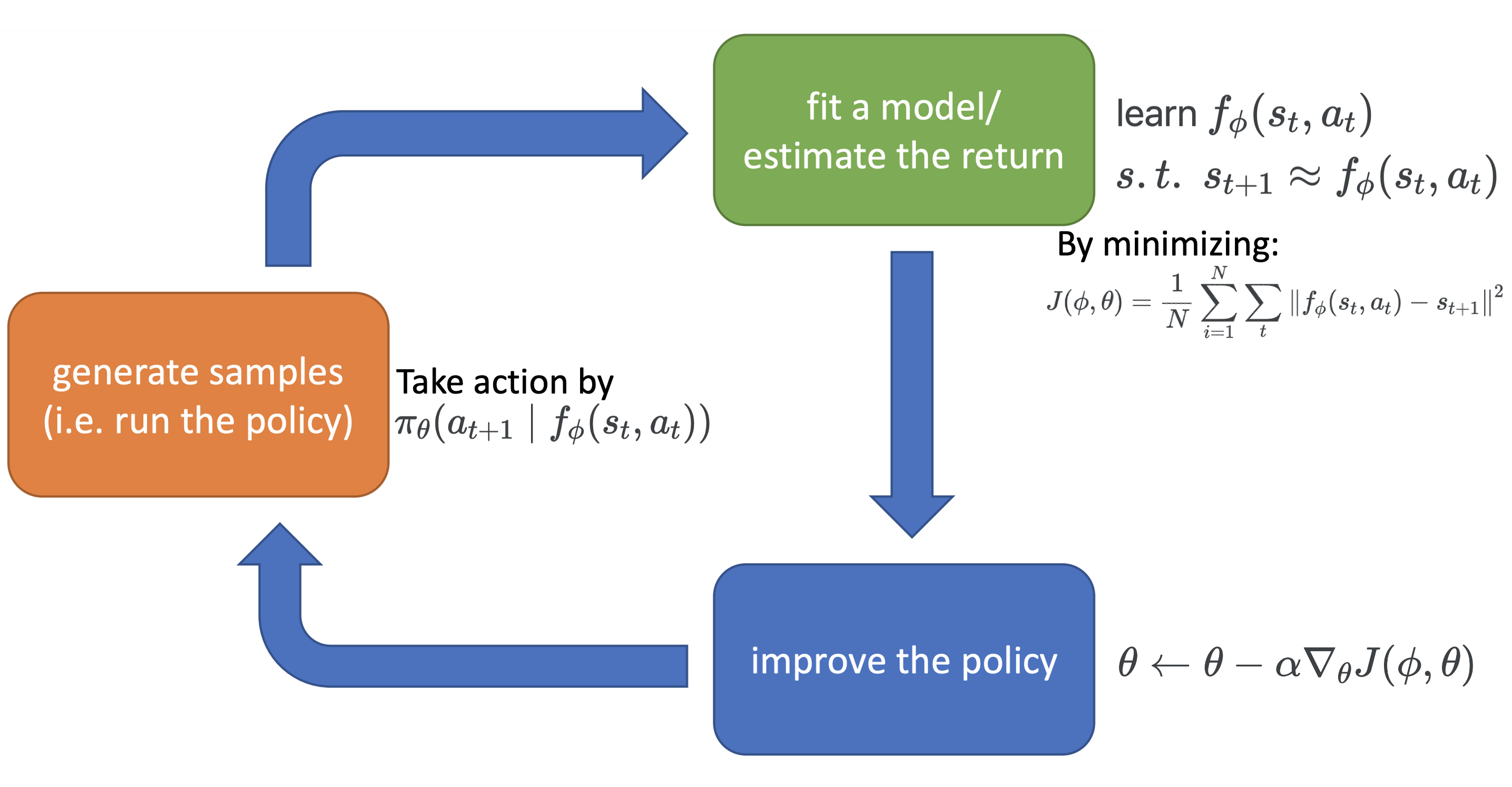
To explain, there are two learnable components in the algorithm — the transition model \(f_{\phi}(s_t, a_t)\), and policy \(\pi_{\theta}\). The objective is
\[\begin{equation} J(\phi,\theta) = \frac1N\sum_{i=1}^N\sum_t \left\|f_{\phi}(s_t, a_t) - s_{t+1}\right\|^2 \end{equation}\]You might wonder why is the objective a function of \(\theta\)? This is because action \(a_t\sim \pi_{\theta}(a_t\mid f_{\phi}(s_{t-1}, a_{t-1}))\). However, differentiating \(J(\phi, \theta)\) w.r.t. \(\theta\) is not straightforward, as sampling is involved in the computation. Luckily, people have developed varies tricks such as the reparameterization trick to handle differentiation through sampling. In fact, here we assume the transition model \(f_{\phi}(s_{t-1}, a_{t-1})\) is deterministic, but it can also be a distribution \(p_{\theta}(s_t\mid s_{t-1}, a_{t-1})\), in which case obtaining the gradient w.r.t \(\phi\) also involves differentiation through sampling.
Don’t worry if any of the above is not clear to you, we will cover these algorithms in later lectures.
Now let’s talk about the three boxes in turns of which is expensive and which is cheap. First of all, as I said before, the complexity of three boxes in different algorithms are different, but it is always true that the orange box is expensive if the algorithm is running in real world, i.e. the robot is operating and collecting data in the real world. But we also have all sorts of simulator which can (drastically) speed up the process. However, there is an inevitable gap between the simulator and the really world (Can we build a simulator that is exactly the same as the real world? That’s impossible for now, because this means we have a perfect model of how the world operates)
How about the green box? For policy gradient, it’s just a summation over rewards, which is very fast, but for model-based policy learning, we need to do gradient update to learn the model, which is more expensive than just summation. For the blue box, policy gradient will do gradient update, while even though model-based policy leraning is also doing gradient update here, it’s more expensive, because the gradient is calculated by backpropagation through time (the first decision affect all later states, the second decision affect all but first state etc. The process is recursive).
3.3 Examples of Value-based Methods and the Actor-critic Algorithm
Finally, there is another type of algorithms that doesn’t not explicitly specify the policy \(\pi_{\theta}\) called value-based methods. We will discuss this type of methods in detail in future lectures, but here let me briefly introduce the key concepts and ideas.
Let’s take a look at the goal of reinforcement learning:
\[\begin{equation}\label{goal2}\text{argmax} \mathbb{E}_{p(\tau)}\sum_{t=1}^T r(s_t, a_t)\end{equation}\]Note that we take \(\theta\) out from the trajectory distribution to indicate that we do not specify a parametric policy \(\pi_{\theta}\). Value-based methods provide a different way to to the maximization.
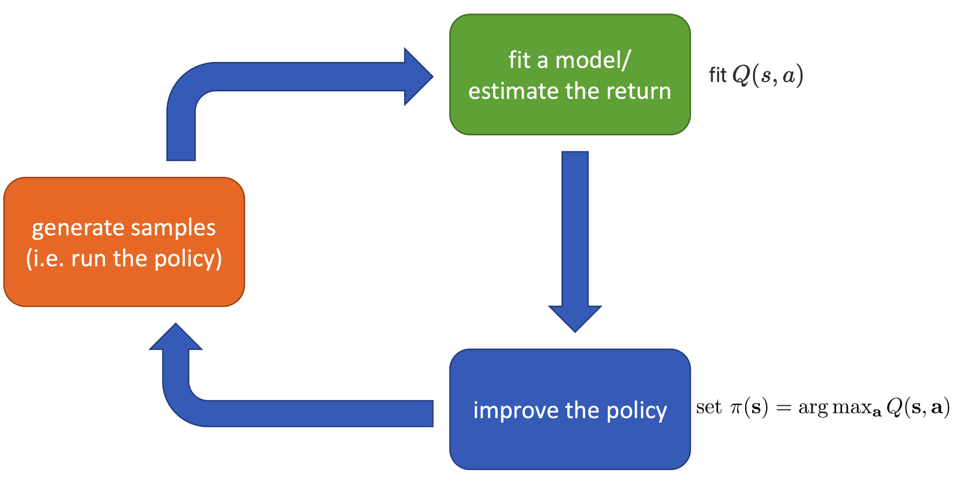
We define Q-function
\[\begin{align} Q(s_t,a_t) &= \mathbb{E}_{p_{\theta}}\left[\sum_{t'=t}^{T}r(s_{t'},a_{t'}) \mid s_t, a_t \right] \\ &= r(s_t, a_t) + \mathbb{E}_{a_{t+1} \sim \pi_{\theta}(a_{t+1}\mid s_{t+1}),s_{t+1}\sim p(s_{t+1}\mid s_t, a_t)} \left[ Q(s_{t+1}, a_{t+1}) \right] \end{align}\]which is the expected reward to go from step \(t\) given the state and action at current state \((s_t, a_t)\). Q-function measures how good the state and action is. Now the goal (equation \(\ref{goal2}\)) can be writen as
\[\begin{equation}\label{one_step} \text{argmax} \mathbb{E}_{s_1 \sim p(s_1)}\left[ \mathbb{E}_{a_1 \sim \pi(a_1\mid s_1)}Q(s_1, a_1) \right] \end{equation}\]In practice, we will know the first state \(s_1\), and if we also know the Q-function \(Q(s_1, a_1)\), we can directly let \(a_1^* = \text{argmax}_{a_1}Q(s_1, a_1)\) and set \(\pi(a_1\mid s_1) = \delta_{a_1^*}(s_1)\). This will give the maximal sum of reward. Therefore, if we know the Q-function at every time step, we can directly take the action that maximize the Q-function, and no parametric policy is needed. However, we will not be able to know the Q-function, how to deal with this? We will discuss some solutions in the later lectures. The following plot shows how this idea fit to our framework.
In addition to the Q-fuction, we can also define the value function:
\[\begin{align} V(s_t) & = \mathbb{E}_{p_{\theta}}\left[\sum_{t'=t}^{T}r(s_{t'},a_{t'}) \mid s_t \right] \\ &= \mathbb{E}_{a_t\sim \pi_{\theta}(a_t\mid s_t)} \left\{ r(s_t, a_t) + \mathbb{E}_{s_{t+1} \sim p(s_{t+1}\mid s_t, a_t)}\left[ V(s_{t+1}) \right] \right\} \end{align}\]Value function measures how good the state is (i.e. the value of the state) First notice that Q-function and value function are related by
\[\begin{equation}\label{relation}V(s_t) = \mathbb{E}_{a_t\sim \pi(a_t\mid s_t)}Q(s_t, a_t)\end{equation}\]Equation \(\ref{relation}\) gives the a nice intuition about Q-function and value function — value function evaluates on average how different actions at the the current state is. This leads to another idea improve the explicit policy — we improve policy \(\pi_{\theta}\) such that the actions taken by running the policy is better than average, i.e. the probability that \(Q(s_t, a_t) > V(s_t)\) is high. This leads to the actor-critic algorithm which stands at the intersection of policy gradient methods and value-based methods. Note that we can also derive Q-function from value function:
\[\begin{equation} Q(s_t, a_t) = r(s_t, a_t) + \mathbb{E}_{s_{t+1} \sim p(s_{t+1}\mid s_t, a_t)}V(s_{t+1})\end{equation}\]The actor-critic algorithm looks like the following in our framework:
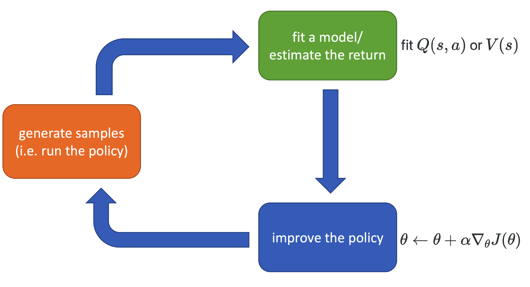
(\(J(\theta)\) is some objective which we optimize to encourage the policy to take actions that are better than average, i.e. \(Q(s_t, a_t) > V(s_t)\))
4 Summary of RL algorithms
In the above section, we have actually introduce examples/ideas of the four main RL algorithms, namely policy gradient methods, value based methods, actor-critic methods, and model-based methods, the first question you might have is, why do we need all these different methods? The is a quite common one, there is no silver bullet. Different algorithms have different assumptions and tradeoffs, so for different RL problems different algorithms might be favourable.
In this section, we discuss the three main considerations when applying RL algorithms, namely assumptions, stability, and sample efficiency. We will not touch any of the mathematical theories behind these properties, some of them will be introduced in future lectures, but this is not a RL theory course, and if you want a full feast of theory, I recommend the book by Agarwal et al.
Also I personally find this part to be hard to follow when I watching the videos, because there are so many terminologies that are not defined at this point of the course. But most of them sense to me now as I have finished learning the course and did all the homeworks. So if you are confused about this part, you can take a quick pass, and maybe come back to it once you finish the whole course.
4.1 Assumptions
- Full observability
- What is it? The state sequence \((s_1, s_2, \cdots)\) is observable, or put it in an other way, the observation sequence \((o_1, o_2, \cdots)\) satisfy markov assumption.
- What algo requires it? Generally required by value function fitting methods. This requirement can be mitigated by adding recurrence and memory.
- Episodic learning
- What is it? The MDP runs for finite amount of time, i.e. trajactory is \((s_1, a_1, \cdots, s_T, a_T)\) and \(T < \infty\). Continuous learning means the task never ends.
- What algo requires it? It is often assumed by pure policy gradient methods, and also assumed by some model-based RL methods. For value-based methods, it’s usually not a necessary assumption, but them tend to work the best when this assumption satisfies.
- Continuity or smoothness of the model
- What is it? The model \(p(s_{t+1}\mid s_t, a_t)\) is continues or smooth in it’s variables.
- What algo requires it? This is often required by model-based algorithms derived from optimal control. This is also assumed by some some continuous value function learning methods.
4.2 Stability
Almost all RL algorithms we will discuss in this course are composed of iterative procedures, and therefore we always want to ask two questions: does the algorithm converge? does the final result of the algorithm gives a higher expected of reward?
Unlike deep supervised learning, RL algorithms are not always gradient descent. For example, the value-based method Q-learning is a fixed point iteration algorithm. Therefore, we cannot just plug in convergence analysis of SGD methods when analyzing RL algorithms;
Unlike deep supervised learning, RL algorithms are not always running towards the goal. For example, model-based RL algorithms fit the model which is not optimized for better expected reward. Therefore, sometimes convergence of a algorithm does not necessarily lead to a better policy.
Policy gradient method is actually directly optimizing for better expected reward via stochastic gradient descent, but sometimes it’s the least efficient algorithm :( This brings us to the last point — sample efficiency.
4.3 Sample efficiency
This is a very important issue in reinforcement learning. In plain english, sample efficiency means how many samples do we need to get a good policy. And the discussion of sample efficiency leads to two categories of methods: on-policy methods and off-policy methods.
On-policy means during training, each time the policy is changed, new samples (i.e. training trajectories) needs to be generated. For example, the classic policy gradient method is an on-policy algorithm, everytime you take one gradient step in the blue box, you need we generate new samples in the orange box to estimate the expected rewards in order for the algorithm to be valid. On-poicy algorithms are generally not very sample efficient.
Off-policy means samples does not need to be generated using the current policy, so off-policy methods are generally more sample efficient. Model-based methods are usually off-policy.
A spectrum of different algorithms in terms of sample efficiency is shown below:
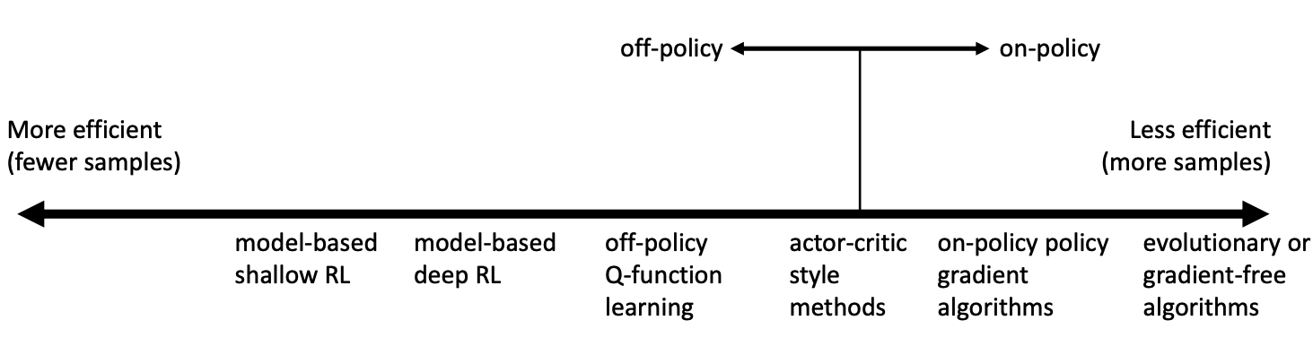
You might ask: why would we use a less sample efficient algorithm? The answer is, wall clock time is not the same as sample efficiency. In some cases, such as playing games, simulator can generate sample very fast and most of the time cost is in updating the policy or updating the model.
Finally, let me introduce a few algorithms under each category.
- Value function fitting methods
- Q-learning, DQN
- Temporal difference learning
- Fitted value iteration
- Policy gradient methods
- REINFORCE
- Natural policy gradient
- Trust region policy optimization
- Actor-critic algorithms
- Advantage actor-critic (A2C)
- Asynchronous advantage actor-critic (A3C)
- Soft actor-critic (SAC)
- Model-based RL algorithms
- Dyna
- Guided policy search
You might notice some famous algorithms above, for example, DQN, which is famous for mastering Atari games (e.g. “Breakout”); or A2C, which is underlying algorithm for the famous AlphaGo. In the rest of this course, we will learn most of the algorithms shown above and many more!